On the Role of Scene Graphs in Image Captioning

29

On the Role of Scene Graphs in Image Captioning

Dalin Wang Daniel Beck Trevor Cohn

School of Computing and Information Systems The University of Melbourne

[email protected]

{d.beck,t.cohn}@unimelb.edu.au

Abstract

Scene graphs represent semantic information in images, which can help image captioning system to produce more descriptive outputs versus using only the image as context. Re-cent captioning approaches rely on ad-hoc ap-proaches to obtain graphs for images. How-ever, those graphs introduce noise and it is un-clear the effect of parser errors on captioning accuracy. In this work, we investigate to what extent scene graphs can help image captioning. Our results show that a state-of-the-art scene graph parser can boost performance almost as much as the ground truth graphs, showing that the bottleneck currently resides more on the captioning models than on the performance of the scene graph parser.

1 Introduction

The task of automatically recognizing and describ-ing visual scenes in the real world, normally re-ferred to as image captioning, is a long stand-ing problem in computer vision and computational linguistics. Previously proposed methods based on deep neural networks have demonstrated convinc-ing results in this task, (Xu et al.,2015;Lu et al.,

2018;Anderson et al., 2018;Lu et al., 2017;Fu et al.,2017;Ren et al.,2017) yet they often pro-duce dry and simplistic captions, which lack de-scriptive depth and omit key relations between ob-jects in the scene. Incorporating complex visual relations knowledge between objects in the form of scene graphs has the potential to improve cap-tioning systems beyond current limitations.

Scene graphs, such as the ones present in the Visual Genome dataset (Krishna et al.,2017), can be used to incorporate external knowledge into images. Because of the structured abstraction and greater semantic representation capacity than purely image features, they have the potential to

improve image captioning, as well as other down-stream tasks that rely on visual components. This has led to the development of many parsing algo-rithms for scene graphs (Li et al.,2018,2017;Xu et al.,2017;Dai et al.,2017;Yu et al.,2017). Si-multaneously, recent work also aimed at incorpo-rating scene graphs into captioning systems, with promising results (Yao et al., 2018; Xu et al.,

2019). However, these previous work still rely on ad-hoc scene graph parsers, raising the question of how captioning systems behave under potential parsing errors.

In this work, we aim at answering the follow-ing question: “to what degree scene graphs con-tribute to the performance of image captioning systems?”. In order to answer this question we provide two contributions: 1) we investigate the performance of incorporating scene graphs gener-ated by a state-of-the-art scene graph parser (Li et al., 2018) into a well-established image cap-tioning framework (Anderson et al.,2018); and 2) we provide an upper bound on the performance by comparative experiments with ground truth graphs. Our results show that scene graphs can be used to boost performance of image captioning, and scene graphs generated by state-of-art scene graph parser, though still limited in the number of objects and relations categories, is not far below the ground-truth graphs, in terms of standard im-age captioning metrics.

2 Methods

Our architecture, inspired by Anderson et al.

Car

Skis Person

Road Tree

Child Skis next to

on on in front of

wearing wearing

scene graph parser

region detector

graph conv net

(GCN)

image region

encoding

att att

<s> a group of

people

attention LSTM

decoder LSTM

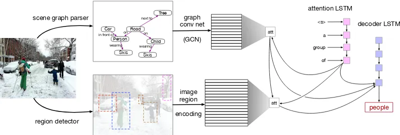
Figure 1: Overview of our architecture for image captioning.

Section 3.1. Given those inputs, our model con-sists a scene graph encoder, an LSTM-based at-tention module and another LSTM as the decoder.

2.1 Scene Graph Encoder

The scene graph is represented as a set of node embeddings which are then updated into contex-tual hidden vectors using a Graph Convolutional Network (Kipf and Welling,2017, GCN). In par-ticular, we employ the GCN version proposed by

Marcheggiani and Titov (2017), who incorporate directions and edge labels. We treat each relation and object in the scene graph as nodes, which are then connected with five different types of edges.1 Since we assume scene graphs are obtained by a parser, they may contain noise in the form of faulty or nugatory connections. To mitigate the influence of parsing errors, we allow edge-wise gating so the network learns to prune those connections. We re-fer toMarcheggiani and Titov(2017) for details of their GCN architecture.

2.2 Attention LSTM

The Attention LSTM keeps track of contextual in-formation from the inputs and incorporates infor-mation from the decoder. At each time stept, the Attention LSTM takes in contextual information by concatenating the previous hidden state of the Decoder LSTM, the mean-pooled region-level im-age features, the mean-pooled scene graph node features from the GCN and the previous gener-ated word representation:x1_t = [h2_t−1,v,f, Weut]

where We is the word embedding matrix for

vo-cabularyΣandut is the one-hot encoding of the

word at time stept. Given the hidden state of the

1_{We use the following types:}

subjindicates the edge be-tween a subject and predicate,objdenotes the edge between a predicate and an object,subj’andobj’, their corresponding reverse edges, and lastly,self, which denotes a self loop.

Attention LSTMh1_t, we generate cascaded atten-tion features, first over scene graph features, and then we concatenate the attention weighted scene graph features with the hidden state of the Atten-tion LSTM to attend over region-level image fea-tures. Here, we only show the second attention step over region-level image features as they are identical procedures except for the input:

bi,t =wTbReLU(Wf bvi+Whb[h1t,ˆft])

βt=softmax(bt); vˆt=

Nv

X

i=1

βi,tvi

wherewT_b ∈RH, Wf b ∈ RH×Df_{, W}

hb ∈RH×H

are learnable weights. vˆtandˆft are the attention

weighted image features and scene graph features respectively.

2.3 Decoder LSTM

The inputs to the Decoder LSTM consist of the previous hidden state from the Attention LSTM layer, attention weighted scene graph node fea-tures, and attention weighted image features.x2_t = [h1_t,ˆft,vˆt] Using the notation y1:T to refer to

a sequence of words (y1, ..., yT) at each time

step t, the conditional distribution over possi-ble output words is given by: p(yt|y1:t−1) =

softmax(Wph2t +bp) where Wp ∈ R|Σ|×H and

bp ∈R|Σ|are learned weights and biases.

2.4 Training and Inference

3 Experiments

Datasets MS-COCO, (Lin et al., 2014) is the most popular benchmark for image captioning, which contains 82,783 training images and 40,504 validation images, with five human-annotated de-scriptions per image. As the annotations of the official testing set are not publicly available, we follow the widely used Kaparthy split ( Karpa-thy and Fei-Fei,2017), and take 113,287 images for training, 5K for validation, and 5K for test-ing. We convert all the descriptions in training set to lower case and discard rare words which oc-cur less than five times, resulting in a vocabulary with 10,201 unique words. For the oracle experi-ments, we take a subset of MS-COCO that inter-sects with Visual Genome (Krishna et al.,2017) to obtain the ground truth scene graphs. The result-ing dataset (henceforth, MS-COCO-GT) contains 33,569 training, 2,108s validation, and 2,116 test images respectively.

Preprocessing The scene graphs are obtained by a state-of-the-art parser: a pre-trained Factorizable-Net trained on MSDN split (Li et al.,

2017), which is a cleaner version of the Visual Genome2 that consists of 150 object categories and 50 relationship categories. Notice that the number of object categories and relationships are much smaller than the actual number of objects and relationships in the Visual Genome dataset. All the predicted objects are associated with a set of bound box coordinates. The region-level image features3 are obtained from Faster-RCNN (Ren et al.,2017), which is also trained on Visual Genome, using 1,600 object classes and 400 at-tributes classes.

Implementation Our models are trained with AdamMax optimizer (Kingma and Ba,2015). We set the initial learning rate as 0.001 with a mini-batch size as 256. We set the maximum number of epochs to be 100 with early stopping mechanism.4 During inference, we set the beam width to 5. Each word in the sentence is represented as a one-hot vector, and each word embedding is a

1,024-2

The MSDN split might contain training instances that overlap with the Karpathy split

3_{These regions are different to those from the scene graph.}

To help the model learn to match regions, the inputs to atten-tion include bounding box coordinates.

4_{We stop training if the CIDEr score does not improve for}

10 epochs, and we reduce the learning by 20 percent if the CIDEr score does not improve for 5 epochs.

B M R C S

No edge-wise gating

I 34.1 26.5 55.5 108.0 19.9

G 22.8 20.6 46.7 66.3 13.5

I+G 34.2 26.5 55.7 108.2 20.1

With edge-wise gating

G 22.9 21.1 47.5 70.7 14.0

I+G 34.5 26.8 55.9 108.6 20.3

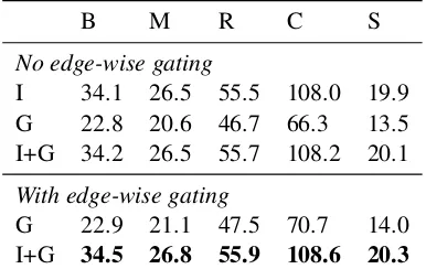
Table 1: Results on the full MS-COCO dataset. “I”, “G” and “I+G” correspond to models using image fea-tures only, scene graphs only and both, respectively. “B”, “M”, “R”, “C” and “S” correspond to BLEU, ME-TEOR, ROUGE, CIDEr and SPICE (higher is better).

dimensional vector. For each image, we have K = 36region features with bounding box coor-dinates from Faster-RCNN. Each region-level im-age feature is represented as a 2,048-dimensional vector, and we concatenate the bounding box coor-dinates to each of the region-level image features. The dimension of the hidden layer in each LSTM and GCN layer is set to 1,024. We use two GCN layers in all our experiments.

Evaluation We employ standard automatic eval-uation metrics including BLEU (Papineni et al.,

2002), METEOR (Lavie and Agarwal, 2007), ROUGE (Lin, 2004), CIDEr (Vedantam et al.,

2015) and SPICE (Anderson et al.,2016), and we use the coco-caption tool5to obtain the scores.

3.1 Quantitative Results and Analysis

Table 1 shows the performances of our mod-els against baseline modmod-els whose architecture is based on Bottom-up Top-down Attention model (Anderson et al., 2018). Overall, our proposed model incorporating scene graph features achieves better results across all evaluation metrics, com-pared to image features only or graph features only. The results show that our model can learn to exploit the relational information in scene graphs and effectively integrate those with image fea-tures. Moreover, the results also demonstrate the effectiveness of edge-wise gating in pruning noisy scene graph features.

We also conduct experiments comparing Factorizable-Net generated scene graph with ground-truth scene graph, as shown in Table2. As expected, the results show that the performance is

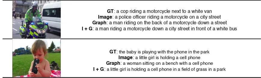
GT: a cop riding a motorcycle next to a white van Image: a police officer riding a motorcycle on a city street Graph: a man riding on the back of a motorcycle down a street I + G: a man riding a motorcycle down a city street in front of a white bus

GT: the baby is playing with the phone in the park

Image: a little girl is holding a cell phone

Graph: a woman sitting on a bench with a cell phone

I + G: a little girl is holding a cell phone in a field of grass in a park

Figure 2: Caption generation results on COCO dataset. All results are generated by models trained on the full ver-sion of Karpathy split, and all graph features are processed by GCN with edge-wise gating. 1) Ground Truth(GT) 2) Image features only(Image) 3) Graph features only(Graph) 4) Ours: Image features plus graph features (I + G)

B M R C S

I 32.0 25.6 54.3 102.2 19.0

G (pred) 17.4 16.5 41.3 49.5 10.6

G (truth) 18.4 17.9 42.5 50.8 11.2

I+G (pred) 32.2 25.8 54.4 103.4 19.1 I+G (truth) 32.5 26.1 54.8 105.2 19.5

Table 2: Results on the MS-COCO-GT dataset.

“G (pred)” refers to the parsed scene graphs from Factorizable-Net while “G (truth)” corresponds to the ground truth graphs obtained from Visual Genome.

better with ground-truth scene graph. Notably the SPICE score, which measures the semantic cor-relation between generated captions and ground truth captions, improved by 2.1%, since there are considerably more types of objects, relations and attributes present in the ground-truth scene graphs. Overall, the results show the potential of incorporating automatically generated scene graph features for the captioning system, and we argue with better scene graph parser trained on more objects, relations and attributes categories, the captioning system should provide additional improvements.

Compared to a recent image captioning paper6 (Li and Jiang, 2019) using scene-graph features, our results are superior, demonstrating the effec-tiveness of our model. Moreover, compared to a state-of-art image captioning system (Yu et al.,

2019),7 our scores are inferior, as we do not ap-ply scheduled sampling, reinforcement learning,

6_{The Hierarchical Attention Model incorporating}

scene-graph features reports scores: Bleu4 33.8, METEOR 26.2, ROUGE 54.9, CIDEr 110.3, SPICE 19.8

7_{This transformer-based captioning system reports scores:}

Bleu4 40.4, METEOR 29.4, ROUGE 59.6, CIDEr 130.0.

transformer cell or ensemble predictions, which have all been proven to improve the scores sig-nificantly. However, our method of incorporating scene-graph features is orthogonal to the state-of-art methods.

3.2 Qualitative Results and Analysis

Figure2shows some generated captions by differ-ent approaches trained on the full Karpathy split of MS-COCO dataset. We can see that all ap-proaches can produce sensible captions describing the image content. However, our approach of in-corporating scene graph features and image fea-tures can generate more descriptive captions that more closely narrate the underlying relations in the image. In the first example, our model correctly predicts that the motercycle is in front of the white van while the image-only model misses this rela-tional detail. On the other hand, purely graph fea-tures sometimes introduce noise. As shown in the second example, the graph-only model mistakes the little girl in a park as a woman on a bench, whereas the image features in our model helps dis-ambiguate faulty graph features.

4 Conclusion

end-to-end multi-task framework that jointly pre-dicts visual relations and captions.

References

Peter Anderson, Basura Fernando, Mark Johnson, and Stephen Gould. 2016. SPICE: semantic proposi-tional image caption evaluation. InComputer Vision - ECCV 2016 - 14th European Conference, Amster-dam, The Netherlands, October 11-14, 2016, Pro-ceedings, Part V, pages 382–398.

Peter Anderson, Xiaodong He, Chris Buehler, Damien Teney, Mark Johnson, Stephen Gould, and Lei Zhang. 2018. Bottom-up and top-down attention for image captioning and visual question answering. In

2018 IEEE Conference on Computer Vision and Pat-tern Recognition, CVPR 2018, Salt Lake City, UT, USA, June 18-22, 2018, pages 6077–6086.

Bo Dai, Yuqi Zhang, and Dahua Lin. 2017. Detecting visual relationships with deep relational networks. In 2017 IEEE Conference on Computer Vision and Pattern Recognition, CVPR 2017, Honolulu, HI, USA, July 21-26, 2017, pages 3298–3308.

Kun Fu, Junqi Jin, Runpeng Cui, Fei Sha, and Chang-shui Zhang. 2017. Aligning where to see and what to tell: Image captioning with region-based atten-tion and scene-specific contexts. IEEE Trans. Pat-tern Anal. Mach. Intell., 39(12):2321–2334.

Andrej Karpathy and Li Fei-Fei. 2017. Deep visual-semantic alignments for generating image descrip-tions. IEEE Trans. Pattern Anal. Mach. Intell., 39(4):664–676.

Diederik P. Kingma and Jimmy Ba. 2015. Adam: A method for stochastic optimization. In 3rd Inter-national Conference on Learning Representations, ICLR 2015, San Diego, CA, USA, May 7-9, 2015, Conference Track Proceedings.

Thomas N. Kipf and Max Welling. 2017.

Semi-supervised classification with graph convolutional networks. In 5th International Conference on Learning Representations, ICLR 2017, Toulon, France, April 24-26, 2017, Conference Track Pro-ceedings.

Ranjay Krishna, Yuke Zhu, Oliver Groth, Justin John-son, Kenji Hata, Joshua Kravitz, Stephanie Chen, Yannis Kalantidis, Li-Jia Li, David A. Shamma, Michael S. Bernstein, and Li Fei-Fei. 2017. Vi-sual genome: Connecting language and vision us-ing crowdsourced dense image annotations. Inter-national Journal of Computer Vision, 123(1):32–73.

Alon Lavie and Abhaya Agarwal. 2007.METEOR: an automatic metric for MT evaluation with high levels of correlation with human judgments. In Proceed-ings of the Second Workshop on Statistical Machine Translation, WMT@ACL 2007, Prague, Czech Re-public, June 23, 2007, pages 228–231.

Xiangyang Li and Shuqiang Jiang. 2019. Know more say less: Image captioning based on scene graphs.

IEEE Trans. Multimedia, 21(8):2117–2130.

Yikang Li, Wanli Ouyang, Bolei Zhou, Jianping Shi, Chao Zhang, and Xiaogang Wang. 2018. Factor-izable net: An efficient subgraph-based framework for scene graph generation. InComputer Vision -ECCV 2018 - 15th European Conference, Munich, Germany, September 8-14, 2018, Proceedings, Part I, pages 346–363.

Yikang Li, Wanli Ouyang, Bolei Zhou, Kun Wang, and Xiaogang Wang. 2017. Scene graph genera-tion from objects, phrases and region capgenera-tions. In

IEEE International Conference on Computer Vision, ICCV 2017, Venice, Italy, October 22-29, 2017, pages 1270–1279.

Chin-Yew Lin. 2004. ROUGE: A package for auto-matic evaluation of summaries. InText Summariza-tion Branches Out, pages 74–81, Barcelona, Spain. Association for Computational Linguistics.

Tsung-Yi Lin, Michael Maire, Serge J. Belongie, James Hays, Pietro Perona, Deva Ramanan, Piotr Doll´ar, and C. Lawrence Zitnick. 2014. Microsoft COCO: common objects in context. In Computer Vision -ECCV 2014 - 13th European Conference, Zurich, Switzerland, September 6-12, 2014, Proceedings, Part V, pages 740–755.

Jiasen Lu, Caiming Xiong, Devi Parikh, and Richard Socher. 2017. Knowing when to look: Adaptive at-tention via a visual sentinel for image captioning. In

2017 IEEE Conference on Computer Vision and Pat-tern Recognition, CVPR 2017, Honolulu, HI, USA, July 21-26, 2017, pages 3242–3250.

Jiasen Lu, Jianwei Yang, Dhruv Batra, and Devi Parikh. 2018. Neural baby talk. In2018 IEEE Con-ference on Computer Vision and Pattern Recogni-tion, CVPR 2018, Salt Lake City, UT, USA, June 18-22, 2018, pages 7219–7228.

Diego Marcheggiani and Ivan Titov. 2017. Encod-ing sentences with graph convolutional networks for semantic role labeling. In Proceedings of the 2017 Conference on Empirical Methods in Natural Language Processing, EMNLP 2017, Copenhagen, Denmark, September 9-11, 2017, pages 1506–1515.

Kishore Papineni, Salim Roukos, Todd Ward, and Wei-Jing Zhu. 2002. Bleu: a method for automatic eval-uation of machine translation. InProceedings of the 40th Annual Meeting of the Association for Compu-tational Linguistics, July 6-12, 2002, Philadelphia, PA, USA., pages 311–318.

Ramakrishna Vedantam, C. Lawrence Zitnick, and Devi Parikh. 2015. Cider: Consensus-based im-age description evaluation. InIEEE Conference on Computer Vision and Pattern Recognition, CVPR 2015, Boston, MA, USA, June 7-12, 2015, pages 4566–4575.

Yonghui Wu, Mike Schuster, Zhifeng Chen, Quoc V. Le, Mohammad Norouzi, Wolfgang Macherey,

Maxim Krikun, Yuan Cao, Qin Gao, Klaus

Macherey, Jeff Klingner, Apurva Shah, Melvin Johnson, Xiaobing Liu, ukasz Kaiser, Stephan

Gouws, Yoshikiyo Kato, Taku Kudo, Hideto

Kazawa, and Jeffrey Dean. 2016. Google’s neural machine translation system: Bridging the gap be-tween human and machine translation.

Danfei Xu, Yuke Zhu, Christopher B. Choy, and Li Fei-Fei. 2017. Scene graph generation by iterative mes-sage passing. In 2017 IEEE Conference on Com-puter Vision and Pattern Recognition, CVPR 2017, Honolulu, HI, USA, July 21-26, 2017, pages 3097– 3106.

Kelvin Xu, Jimmy Ba, Ryan Kiros, Kyunghyun Cho, Aaron C. Courville, Ruslan Salakhutdinov, Richard S. Zemel, and Yoshua Bengio. 2015. Show, attend and tell: Neural image caption generation with visual attention. InProceedings of the 32nd In-ternational Conference on Machine Learning, ICML 2015, Lille, France, 6-11 July 2015, pages 2048– 2057.

Ning Xu, An-An Liu, Jing Liu, Weizhi Nie, and Yuting Su. 2019. Scene graph captioner: Image captioning based on structural visual representation. J. Visual Communication and Image Representation, 58:477– 485.

Ting Yao, Yingwei Pan, Yehao Li, and Tao Mei. 2018.

Exploring visual relationship for image captioning. In Computer Vision - ECCV 2018 - 15th Euro-pean Conference, Munich, Germany, September 8-14, 2018, Proceedings, Part XIV, pages 711–727.

Jun Yu, Jing Li, Zhou Yu, and Qingming Huang. 2019. Multimodal transformer with multi-view vi-sual representation for image captioning. CoRR, abs/1905.07841.