Convolutional Neural Networks for Sentence Classification
Yoon Kim New York University [email protected]
Abstract
We report on a series of experiments with convolutional neural networks (CNN) trained on top of pre-trained word vec-tors for sentence-level classification tasks. We show that a simple CNN with lit-tle hyperparameter tuning and static vec-tors achieves excellent results on multi-ple benchmarks. Learning task-specific vectors through fine-tuning offers further gains in performance. We additionally propose a simple modification to the ar-chitecture to allow for the use of both task-specific and static vectors. The CNN models discussed herein improve upon the state of the art on 4 out of 7 tasks, which include sentiment analysis and question classification.
1 Introduction
Deep learning models have achieved remarkable results in computer vision (Krizhevsky et al., 2012) and speech recognition (Graves et al., 2013) in recent years. Within natural language process-ing, much of the work with deep learning meth-ods has involved learning word vector representa-tions through neural language models (Bengio et al., 2003; Yih et al., 2011; Mikolov et al., 2013) and performing composition over the learned word vectors for classification (Collobert et al., 2011). Word vectors, wherein words are projected from a
sparse, 1-of-V encoding (hereV is the vocabulary
size) onto a lower dimensional vector space via a hidden layer, are essentially feature extractors that encode semantic features of words in their dimen-sions. In such dense representations, semantically close words are likewise close—in euclidean or cosine distance—in the lower dimensional vector space.
Convolutional neural networks (CNN) utilize layers with convolving filters that are applied to
local features (LeCun et al., 1998). Originally invented for computer vision, CNN models have subsequently been shown to be effective for NLP and have achieved excellent results in semantic parsing (Yih et al., 2014), search query retrieval (Shen et al., 2014), sentence modeling (Kalch-brenner et al., 2014), and other traditional NLP tasks (Collobert et al., 2011).
In the present work, we train a simple CNN with one layer of convolution on top of word vectors obtained from an unsupervised neural language model. These vectors were trained by Mikolov et al. (2013) on 100 billion words of Google News,
and are publicly available.1 We initially keep the
word vectors static and learn only the other param-eters of the model. Despite little tuning of hyper-parameters, this simple model achieves excellent results on multiple benchmarks, suggesting that the pre-trained vectors are ‘universal’ feature ex-tractors that can be utilized for various classifica-tion tasks. Learning task-specific vectors through fine-tuning results in further improvements. We finally describe a simple modification to the archi-tecture to allow for the use of both pre-trained and task-specific vectors by having multiple channels. Our work is philosophically similar to Razavian et al. (2014) which showed that for image clas-sification, feature extractors obtained from a pre-trained deep learning model perform well on a va-riety of tasks—including tasks that are very dif-ferent from the original task for which the feature extractors were trained.
2 Model
The model architecture, shown in figure 1, is a slight variant of the CNN architecture of Collobert
et al. (2011). Letxi ∈ Rk be thek-dimensional
word vector corresponding to thei-th word in the
sentence. A sentence of lengthn(padded where
1https://code.google.com/p/word2vec/
wait for the video
and do n't rent
it
n x k representation of sentence with static and
non-static channels
Convolutional layer with multiple filter widths and
feature maps
Max-over-time pooling
Fully connected layer with dropout and
[image:2.595.110.519.61.218.2]softmax output
Figure 1: Model architecture with two channels for an example sentence.
necessary) is represented as
x1:n=x1⊕x2⊕. . .⊕xn, (1)
where ⊕ is the concatenation operator. In
gen-eral, letxi:i+j refer to the concatenation of words
xi,xi+1, . . . ,xi+j. A convolution operation
in-volves a filter w ∈ Rhk, which is applied to a
window ofhwords to produce a new feature. For
example, a featureci is generated from a window
of wordsxi:i+h−1by
ci=f(w·xi:i+h−1+b). (2)
Here b ∈ Ris a bias term and f is a non-linear
function such as the hyperbolic tangent. This filter is applied to each possible window of words in the sentence{x1:h,x2:h+1, . . . ,xn−h+1:n}to produce
afeature map
c= [c1, c2, . . . , cn−h+1], (3)
with c ∈ Rn−h+1. We then apply a
max-over-time pooling operation (Collobert et al., 2011) over the feature map and take the maximum value
ˆ
c = max{c}as the feature corresponding to this particular filter. The idea is to capture the most im-portant feature—one with the highest value—for each feature map. This pooling scheme naturally deals with variable sentence lengths.
We have described the process by which one
feature is extracted from one filter. The model
uses multiple filters (with varying window sizes) to obtain multiple features. These features form the penultimate layer and are passed to a fully con-nected softmax layer whose output is the probabil-ity distribution over labels.
In one of the model variants, we experiment with having two ‘channels’ of word vectors—one
that is kept static throughout training and one that
is fine-tuned via backpropagation (section 3.2).2
In the multichannel architecture, illustrated in fig-ure 1, each filter is applied to both channels and
the results are added to calculate ci in equation
(2). The model is otherwise equivalent to the sin-gle channel architecture.
2.1 Regularization
For regularization we employ dropout on the
penultimate layer with a constraint onl2-norms of
the weight vectors (Hinton et al., 2012). Dropout prevents co-adaptation of hidden units by ran-domly dropping out—i.e., setting to zero—a
pro-portion p of the hidden units during
foward-backpropagation. That is, given the penultimate layerz = [ˆc1, . . . ,ˆcm](note that here we havem
filters), instead of using
y=w·z+b (4)
for output unity in forward propagation, dropout
uses
y=w·(z◦r) +b, (5)
where◦is the element-wise multiplication
opera-tor andr∈Rmis a ‘masking’ vector of Bernoulli
random variables with probability p of being 1.
Gradients are backpropagated only through the unmasked units. At test time, the learned weight
vectors are scaled by p such that wˆ = pw, and
ˆ
wis used (without dropout) to score unseen
sen-tences. We additionally constrainl2-norms of the
weight vectors by rescalingwto have||w||2 = s
whenever||w||2 > safter a gradient descent step.
Data c l N |V| |Vpre| Test
MR 2 20 10662 18765 16448 CV
SST-1 5 18 11855 17836 16262 2210
SST-2 2 19 9613 16185 14838 1821
Subj 2 23 10000 21323 17913 CV TREC 6 10 5952 9592 9125 500
[image:3.595.73.294.62.174.2]CR 2 19 3775 5340 5046 CV MPQA 2 3 10606 6246 6083 CV
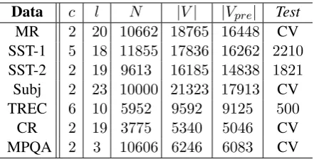
Table 1: Summary statistics for the datasets after tokeniza-tion.c: Number of target classes.l: Average sentence length. N: Dataset size. |V|: Vocabulary size. |Vpre|: Number of
words present in the set of pre-trained word vectors. Test: Test set size (CV means there was no standard train/test split and thus 10-fold CV was used).
3 Datasets and Experimental Setup
We test our model on various benchmarks. Sum-mary statistics of the datasets are in table 1.
• MR: Movie reviews with one sentence per
re-view. Classification involves detecting
posi-tive/negative reviews (Pang and Lee, 2005).3
• SST-1: Stanford Sentiment Treebank—an extension of MR but with train/dev/test splits provided and fine-grained labels (very pos-itive, pospos-itive, neutral, negative, very
nega-tive), re-labeled by Socher et al. (2013).4
• SST-2: Same as SST-1 but with neutral re-views removed and binary labels.
• Subj: Subjectivity dataset where the task is
to classify a sentence as being subjective or objective (Pang and Lee, 2004).
• TREC: TREC question dataset—task
in-volves classifying a question into 6 question types (whether the question is about person, location, numeric information, etc.) (Li and
Roth, 2002).5
• CR: Customer reviews of various products
(cameras, MP3s etc.). Task is to predict
pos-itive/negative reviews (Hu and Liu, 2004).6
3https://www.cs.cornell.edu/people/pabo/movie-review-data/ 4http://nlp.stanford.edu/sentiment/ Data is actually provided at the phrase-level and hence we train the model on both phrases and sentences but only score on sentences at test time, as in Socher et al. (2013), Kalchbrenner et al. (2014), and Le and Mikolov (2014). Thus the training set is an order of magnitude larger than listed in table 1.
5http://cogcomp.cs.illinois.edu/Data/QA/QC/
6http://www.cs.uic.edu/∼liub/FBS/sentiment-analysis.html
• MPQA: Opinion polarity detection subtask
of the MPQA dataset (Wiebe et al., 2005).7
3.1 Hyperparameters and Training
For all datasets we use: rectified linear units, filter
windows (h) of 3, 4, 5 with 100 feature maps each,
dropout rate (p) of 0.5,l2 constraint (s) of 3, and
mini-batch size of 50. These values were chosen via a grid search on the SST-2 dev set.
We do not otherwise perform any dataset-specific tuning other than early stopping on dev sets. For datasets without a standard dev set we randomly select 10% of the training data as the dev set. Training is done through stochastic gra-dient descent over shuffled mini-batches with the Adadelta update rule (Zeiler, 2012).
3.2 Pre-trained Word Vectors
Initializing word vectors with those obtained from an unsupervised neural language model is a popu-lar method to improve performance in the absence of a large supervised training set (Collobert et al., 2011; Socher et al., 2011; Iyyer et al., 2014). We
use the publicly availableword2vecvectors that
were trained on 100 billion words from Google News. The vectors have dimensionality of 300 and were trained using the continuous bag-of-words architecture (Mikolov et al., 2013). Words not present in the set of pre-trained words are initial-ized randomly.
3.3 Model Variations
We experiment with several variants of the model.
• CNN-rand: Our baseline model where all words are randomly initialized and then mod-ified during training.
• CNN-static: A model with pre-trained
vectors from word2vec. All words—
including the unknown ones that are ran-domly initialized—are kept static and only the other parameters of the model are learned.
• CNN-non-static: Same as above but the pre-trained vectors are fine-tuned for each task.
• CNN-multichannel: A model with two sets of word vectors. Each set of vectors is treated as a ‘channel’ and each filter is applied
Model MR SST-1 SST-2 Subj TREC CR MPQA
CNN-rand 76.1 45.0 82.7 89.6 91.2 79.8 83.4
CNN-static 81.0 45.5 86.8 93.0 92.8 84.7 89.6
CNN-non-static 81.5 48.0 87.2 93.4 93.6 84.3 89.5
CNN-multichannel 81.1 47.4 88.1 93.2 92.2 85.0 89.4
RAE (Socher et al., 2011) 77.7 43.2 82.4 − − − 86.4
MV-RNN (Socher et al., 2012) 79.0 44.4 82.9 − − − −
RNTN (Socher et al., 2013) − 45.7 85.4 − − − −
DCNN (Kalchbrenner et al., 2014) − 48.5 86.8 − 93.0 − −
Paragraph-Vec (Le and Mikolov, 2014) − 48.7 87.8 − − − −
CCAE (Hermann and Blunsom, 2013) 77.8 − − − − − 87.2
Sent-Parser (Dong et al., 2014) 79.5 − − − − − 86.3
NBSVM (Wang and Manning, 2012) 79.4 − − 93.2 − 81.8 86.3
MNB (Wang and Manning, 2012) 79.0 − − 93.6 − 80.0 86.3
G-Dropout (Wang and Manning, 2013) 79.0 − − 93.4 − 82.1 86.1
F-Dropout (Wang and Manning, 2013) 79.1 − − 93.6 − 81.9 86.3
Tree-CRF (Nakagawa et al., 2010) 77.3 − − − − 81.4 86.1
CRF-PR (Yang and Cardie, 2014) − − − − − 82.7 −
[image:4.595.73.525.60.325.2]SVMS (Silva et al., 2011) − − − − 95.0 − −
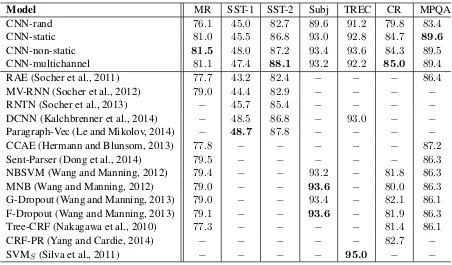
Table 2: Results of our CNN models against other methods.RAE: Recursive Autoencoders with pre-trained word vectors from Wikipedia (Socher et al., 2011). MV-RNN: Matrix-Vector Recursive Neural Network with parse trees (Socher et al., 2012).
RNTN: Recursive Neural Tensor Network with tensor-based feature function and parse trees (Socher et al., 2013). DCNN: Dynamic Convolutional Neural Network with k-max pooling (Kalchbrenner et al., 2014). Paragraph-Vec: Logistic regres-sion on top of paragraph vectors (Le and Mikolov, 2014). CCAE: Combinatorial Category Autoencoders with combinatorial category grammar operators (Hermann and Blunsom, 2013). Sent-Parser: Sentiment analysis-specific parser (Dong et al., 2014).NBSVM, MNB: Naive Bayes SVM and Multinomial Naive Bayes with uni-bigrams from Wang and Manning (2012).
G-Dropout, F-Dropout: Gaussian Dropout and Fast Dropout from Wang and Manning (2013). Tree-CRF: Dependency tree with Conditional Random Fields (Nakagawa et al., 2010).CRF-PR: Conditional Random Fields with Posterior Regularization (Yang and Cardie, 2014).SVMS: SVM with uni-bi-trigrams, wh word, head word, POS, parser, hypernyms, and 60 hand-coded rules as features from Silva et al. (2011).
to both channels, but gradients are back-propagated only through one of the chan-nels. Hence the model is able to fine-tune one set of vectors while keeping the other static. Both channels are initialized with
word2vec.
In order to disentangle the effect of the above variations versus other random factors, we elim-inate other sources of randomness—CV-fold as-signment, initialization of unknown word vec-tors, initialization of CNN parameters—by keep-ing them uniform within each dataset.
4 Results and Discussion
Results of our models against other methods are listed in table 2. Our baseline model with all ran-domly initialized words (CNN-rand) does not form well on its own. While we had expected per-formance gains through the use of pre-trained vec-tors, we were surprised at the magnitude of the gains. Even a simple model with static vectors (CNN-static) performs remarkably well, giving
competitive results against the more sophisticated deep learning models that utilize complex pool-ing schemes (Kalchbrenner et al., 2014) or require parse trees to be computed beforehand (Socher et al., 2013). These results suggest that the pre-trained vectors are good, ‘universal’ feature ex-tractors and can be utilized across datasets. Fine-tuning the pre-trained vectors for each task gives still further improvements (CNN-non-static).
4.1 Multichannel vs. Single Channel Models
Most Similar Words for Static Channel Non-static Channel
bad
good terrible terrible horrible horrible lousy
lousy stupid
good
great nice bad decent terrific solid decent terrific
n’t
os not
ca never
ireland nothing wo neither
!
2,500 2,500 entire lush
jez beautiful changer terrific
,
decasia but abysmally dragon
demise a
valiant and
Table 3: Top 4 neighboring words—based on cosine similarity—for vectors in the static channel (left) and fine-tuned vectors in the non-static channel (right) from the mul-tichannel model on the SST-2 dataset after training.
4.2 Static vs. Non-static Representations
As is the case with the single channel non-static model, the multichannel model is able to fine-tune the non-static channel to make it more specific to
the task-at-hand. For example,goodis most
sim-ilar to bad in word2vec, presumably because
they are (almost) syntactically equivalent. But for vectors in the non-static channel that were fine-tuned on the SST-2 dataset, this is no longer the
case (table 3). Similarly, goodis arguably closer
tonicethan it is togreatfor expressing sentiment,
and this is indeed reflected in the learned vectors. For (randomly initialized) tokens not in the set of pre-trained vectors, fine-tuning allows them to learn more meaningful representations: the net-work learns that exclamation marks are associ-ated with effusive expressions and that commas are conjunctive (table 3).
4.3 Further Observations
We report on some further experiments and obser-vations:
• Kalchbrenner et al. (2014) report much
worse results with a CNN that has essentially
the same architecture as our single channel model. For example, their Max-TDNN (Time Delay Neural Network) with randomly
ini-tialized words obtains 37.4% on the SST-1
dataset, compared to 45.0% for our model.
We attribute such discrepancy to our CNN having much more capacity (multiple filter widths and feature maps).
• Dropout proved to be such a good regularizer
that it was fine to use a larger than necessary network and simply let dropout regularize it. Dropout consistently added 2%–4% relative performance.
• When randomly initializing words not in
word2vec, we obtained slight improve-ments by sampling each dimension from
U[−a, a] where awas chosen such that the
randomly initialized vectors have the same variance as the pre-trained ones. It would be interesting to see if employing more sophis-ticated methods to mirror the distribution of pre-trained vectors in the initialization pro-cess gives further improvements.
• We briefly experimented with another set of
publicly available word vectors trained by
Collobert et al. (2011) on Wikipedia,8 and
found thatword2vecgave far superior
per-formance. It is not clear whether this is due to Mikolov et al. (2013)’s architecture or the 100 billion word Google News dataset.
• Adadelta (Zeiler, 2012) gave similar results
to Adagrad (Duchi et al., 2011) but required fewer epochs.
5 Conclusion
In the present work we have described a series of experiments with convolutional neural networks
built on top of word2vec. Despite little tuning
of hyperparameters, a simple CNN with one layer of convolution performs remarkably well. Our re-sults add to the well-established evidence that un-supervised pre-training of word vectors is an im-portant ingredient in deep learning for NLP.
Acknowledgments
We would like to thank Yann LeCun and the anonymous reviewers for their helpful feedback and suggestions.
[image:5.595.77.287.59.366.2]References
Y. Bengio, R. Ducharme, P. Vincent. 2003. Neu-ral Probabilitistic Language Model. Journal of Ma-chine Learning Research3:1137–1155.
R. Collobert, J. Weston, L. Bottou, M. Karlen, K. Kavukcuglu, P. Kuksa. 2011. Natural Language Processing (Almost) from Scratch. Journal of Ma-chine Learning Research 12:2493–2537.
J. Duchi, E. Hazan, Y. Singer. 2011 Adaptive subgra-dient methods for online learning and stochastic op-timization. Journal of Machine Learning Research, 12:2121–2159.
L. Dong, F. Wei, S. Liu, M. Zhou, K. Xu. 2014. A Statistical Parsing Framework for Sentiment Classi-fication.CoRR, abs/1401.6330.
A. Graves, A. Mohamed, G. Hinton. 2013. Speech recognition with deep recurrent neural networks. In Proceedings of ICASSP 2013.
G. Hinton, N. Srivastava, A. Krizhevsky, I. Sutskever, R. Salakhutdinov. 2012. Improving neural net-works by preventing co-adaptation of feature detec-tors. CoRR, abs/1207.0580.
K. Hermann, P. Blunsom. 2013. The Role of Syntax in Vector Space Models of Compositional Semantics. In Proceedings of ACL 2013.
M. Hu, B. Liu. 2004. Mining and Summarizing
Cus-tomer Reviews. In Proceedings of ACM SIGKDD
2004.
M. Iyyer, P. Enns, J. Boyd-Graber, P. Resnik 2014. Political Ideology Detection Using Recursive Neural Networks.In Proceedings of ACL 2014.
N. Kalchbrenner, E. Grefenstette, P. Blunsom. 2014. A Convolutional Neural Network for Modelling Sen-tences. In Proceedings of ACL 2014.
A. Krizhevsky, I. Sutskever, G. Hinton. 2012. Ima-geNet Classification with Deep Convolutional Neu-ral Networks. In Proceedings of NIPS 2012. Q. Le, T. Mikolov. 2014. Distributed Represenations
of Sentences and Documents. In Proceedings of ICML 2014.
Y. LeCun, L. Bottou, Y. Bengio, P. Haffner. 1998. Gradient-based learning applied to document recog-nition. In Proceedings of the IEEE, 86(11):2278– 2324, November.
X. Li, D. Roth. 2002. Learning Question Classifiers. In Proceedings of ACL 2002.
T. Mikolov, I. Sutskever, K. Chen, G. Corrado, J. Dean. 2013. Distributed Representations of Words and Phrases and their Compositionality. In Proceedings of NIPS 2013.
T. Nakagawa, K. Inui, S. Kurohashi. 2010. De-pendency tree-based sentiment classification using CRFs with hidden variables.In Proceedings of ACL 2010.
B. Pang, L. Lee. 2004. A sentimental education: Sentiment analysis using subjectivity summarization
based on minimum cuts. In Proceedings of ACL
2004.
B. Pang, L. Lee. 2005. Seeing stars: Exploiting class relationships for sentiment categorization with re-spect to rating scales.In Proceedings of ACL 2005. A.S. Razavian, H. Azizpour, J. Sullivan, S. Carlsson
2014. CNN Features off-the-shelf: an Astounding Baseline. CoRR, abs/1403.6382.
Y. Shen, X. He, J. Gao, L. Deng, G. Mesnil. 2014. Learning Semantic Representations Using Convolu-tional Neural Networks for Web Search. In Proceed-ings of WWW 2014.
J. Silva, L. Coheur, A. Mendes, A. Wichert. 2011. From symbolic to sub-symbolic information in ques-tion classificaques-tion. Artificial Intelligence Review, 35(2):137–154.
R. Socher, J. Pennington, E. Huang, A. Ng, C. Man-ning. 2011. Semi-Supervised Recursive Autoen-coders for Predicting Sentiment Distributions. In Proceedings of EMNLP 2011.
R. Socher, B. Huval, C. Manning, A. Ng. 2012. Se-mantic Compositionality through Recursive Matrix-Vector Spaces. In Proceedings of EMNLP 2012. R. Socher, A. Perelygin, J. Wu, J. Chuang, C. Manning,
A. Ng, C. Potts. 2013. Recursive Deep Models for Semantic Compositionality Over a Sentiment Tree-bank.In Proceedings of EMNLP 2013.
J. Wiebe, T. Wilson, C. Cardie. 2005. Annotating Ex-pressions of Opinions and Emotions in Language. Language Resources and Evaluation, 39(2-3): 165– 210.
S. Wang, C. Manning. 2012. Baselines and Bigrams: Simple, Good Sentiment and Topic Classification. In Proceedings of ACL 2012.
S. Wang, C. Manning. 2013. Fast Dropout Training. In Proceedings of ICML 2013.
B. Yang, C. Cardie. 2014. Context-aware Learning for Sentence-level Sentiment Analysis with Poste-rior Regularization.In Proceedings of ACL 2014. W. Yih, K. Toutanova, J. Platt, C. Meek. 2011.
Learn-ing Discriminative Projections for Text Similarity Measures. Proceedings of the Fifteenth Confer-ence on Computational Natural Language Learning, 247–256.
W. Yih, X. He, C. Meek. 2014. Semantic Parsing for Single-Relation Question Answering. In Proceed-ings of ACL 2014.