Convolutional Neural Networks Analyzed via
Convolutional Sparse Coding
Vardan Papyan* [email protected]
Department of Computer Science Technion - Israel Institute of Technology Technion City, Haifa 32000, Israel
Yaniv Romano* [email protected]
Department of Electrical Engineering Technion - Israel Institute of Technology Technion City, Haifa 32000, Israel
Michael Elad [email protected]
Department of Computer Science Technion - Israel Institute of Technology Technion City, Haifa 32000, Israel
Editor:Kevin Murphy
Abstract
Convolutional neural networks (CNN) have led to many state-of-the-art results spanning through various fields. However, a clear and profound theoretical understanding of the forward pass, the core algorithm of CNN, is still lacking. In parallel, within the wide field of sparse approximation, Convolutional Sparse Coding (CSC) has gained increasing attention in recent years. A theoretical study of this model was recently conducted, establishing it as a reliable and stable alternative to the commonly practiced patch-based processing. Herein, we propose a novel multi-layer model, ML-CSC, in which signals are assumed to emerge from a cascade of CSC layers. This is shown to be tightly connected to CNN, so much so that the forward pass of the CNN is in fact the thresholding pursuit serving the ML-CSC model. This connection brings a fresh view to CNN, as we are able to attribute to this architecture theoretical claims such as uniqueness of the representations throughout the network, and their stable estimation, all guaranteed under simple local sparsity conditions. Lastly, identifying the weaknesses in the above pursuit scheme, we propose an alternative to the forward pass, which is connected to deconvolutional and recurrent networks, and also has better theoretical guarantees.
Keywords: Deep Learning, Convolutional Neural Networks, Forward Pass, Sparse Rep-resentation, Convolutional Sparse Coding, Thresholding Algorithm, Basis Pursuit
∗. The authors contributed equally to this work.
c
1. Introduction
Deep learning (LeCun et al., 2015), and in particular CNN (LeCun et al., 1990, 1998; Krizhevsky et al., 2012), has gained a copious amount of attention in recent years as it has led to many state-of-the-art results spanning through many fields – including speech recognition (Bengio et al., 2003; Hinton et al., 2012; Mikolov et al., 2013), computer vision (Farabet et al., 2013; Simonyan and Zisserman, 2014; He et al., 2015), signal and image processing (Gatys et al., 2015; Ulyanov et al., 2016; Johnson et al., 2016; Dong et al., 2016), to name a few. In the context of CNN, the forward pass is a multi-layer scheme that provides an end-to-end mapping, from an input signal to some desired output. Each layer of this algorithm consists of three steps. The first convolves the input with a set of learned filters, resulting in a set of feature (or kernel) maps. These then undergo a point wise non-linear function, in a second step, often resulting in a sparse outcome (Glorot et al., 2011). A third (and optional) down-sampling step, termedpooling, is then applied on the result in order to reduce its dimensions. The output of this layer is then fed into another one, thus forming the multi-layer structure, often termed forward pass.
Despite its marvelous empirical success, a clear and profound theoretical understanding of this scheme is still lacking. A few preliminary theoretical results were recently sug-gested. In (Mallat, 2012; Bruna and Mallat, 2013) the Scattering Transform was proposed, suggesting to replace the learned filters in the CNN with predefined Wavelet functions. In-terestingly, the features obtained from this network were shown to be invariant to various transformations such as translations and rotations. Other works have studied the properties of deep and fully connected networks under the assumption of independent identically dis-tributed random weights (Giryes et al., 2015; Saxe et al., 2013; Arora et al., 2014; Dauphin et al., 2014; Choromanska et al., 2015). In particular, in (Giryes et al., 2015) deep neural networks were proven to preserve the metric structure of the input data as it propagates through the layers of the network. This, in turn, was shown to allow a stable recovery of the data from the features obtained from the network.
afore-mentioned limitations by imposing a special structure – a union of banded and Circulant matrices – on the dictionary involved. The traditional sparse model has been extensively studied over the past two decades (Elad, 2010; Foucart and Rauhut, 2013). More recently, the convolutional extension was extensively analyzed in (Papyan et al., 2016a,b), shedding light on its theoretical aspects and prospects of success.
In this work, by leveraging the recent study of CSC, we aim to provide a new perspec-tive on CNN, leading to a clear and profound theoretical understanding of this scheme, along with new insights. Embarking from the classic CSC, our approach builds upon the observation that similar to the original signal, the representation vector itself also admits a convolutional sparse representation. As such, it can be modeled as a superposition of atoms, taken from a different convolutional dictionary. This rationale can be extended to several layers, leading to the definition of our proposed ML-CSC model. Building on the recent analysis of the CSC, we provide a theoretical study of this novel model and its associated pursuits, namely the layered thresholding algorithm and the layered basis pursuit (BP).
Our analysis reveals the relation between the CNN and the ML-CSC model, showing that the forward pass of the CNN is in fact identical to our proposed pursuit – the layered thresholding algorithm. This connection is of significant importance since it gives a clear mathematical meaning, objective and model to the CNN architecture, which in turn can be accompanied by guarantees for the success of the forward pass, studied via the layered thresholding algorithm. Specifically, we show that the forward pass is guaranteed to recover an estimate of the underlying representations of an input signal, assuming these are sparse in a local sense. Moreover, considering a setting where a norm-bounded noise is added to the signal, we show that such a mild corruption in the input results in a bounded perturbation in the output – indicating the stability of the CNN in recovering the underlying representations. Lastly, we exploit the answers to the above questions in order to propose an alternative to the commonly used forward pass algorithm, which is tightly connected to both deconvolutional (Zeiler et al., 2010; Pu et al., 2016) and recurrent networks (Bengio et al., 1994). The proposed alternative scheme is accompanied by a thorough theoretical study. Although this and the analysis presented throughout this work focus on CNN, we will show that they also hold for fully connected networks.
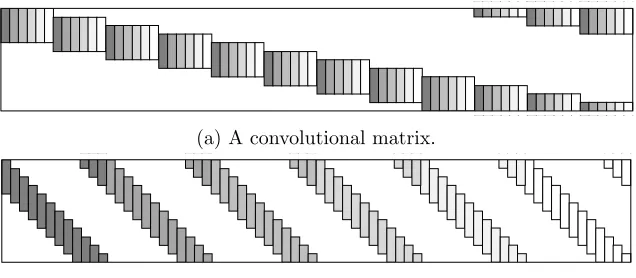
(a) A convolutional matrix.
(b) A concatenation of banded and Circulant matrices.
Figure 1: The two facets of the convolutional structure.
2. Background
This section is divided into two parts: The first is dedicated to providing a simple mathemat-ical formulation of the CNN and the forward pass, while the second reviews the Sparse-Land model and its various extensions. Readers familiar with these two topics can skip directly to Section 3, which moves to serve the main contribution of this work.
2.1 Deep Learning - Convolutional Neural Networks
The fundamental algorithm of deep learning is the forward pass, employed both in the training and the inference stages. The first step of this algorithm convolves an input (one dimensional) signalX∈RN with a set ofm1 learned filters of lengthn0, creatingm1feature (or kernel) maps. Equally, this convolution can be written as a matrix-vector multiplication, W1TX∈RN m1, where W
1 ∈RN×N m1 is a matrix containing in its columns the m1 filters with all of their shifts. This structure, also known as a convolutional matrix, is depicted in Figure 1a. A pointwise nonlinear function is then applied on the sum of the obtained feature mapsWT1Xand a bias term denoted byb1 ∈RN m1. Many possible functions were proposed
over the years, the most popular one being the Rectifier Linear Unit (ReLU) (Glorot et al., 2011; Krizhevsky et al., 2012), formally defined as ReLU(z) = max(z,0). By cascading the basic block of convolutions followed by a nonlinear function, Z1 = ReLU(WT1X+b1), a multi-layer structure of depth K is constructed. Formally, for two layers this is given by
f(X,{Wi}2i=1,{bi}2i=1) =Z2= ReLU
W2T ReLU WT1X+b1
+b2
, (1)
where W2 ∈ RN m1×N m2 is a convolutional matrix (up to a small modification discussed
below) constructed from m2 filters of length n1m1 and b2 ∈ RN m2 is its corresponding
bias. Although the two layers considered here can be readily extended to a much deeper configuration, we defer this to a later stage.
By changing the order of the columns in the convolutional matrix, one can observe that it can be equally viewed as a concatenation of banded and Circulant1 matrices, as depicted 1. We shall assume throughout this paper that boundaries are treated by a periodic continuation, which
𝑚1
𝐖2T∈ ℝ𝑁𝑚2×𝑁𝑚1
𝐖1T ∈ ℝ𝑁𝑚1×𝑁
𝐗 ∈ ℝ𝑁 𝐛1∈ ℝ𝑁𝑚1
𝐛2∈ ℝ𝑁𝑚2 𝐙2∈ ℝ𝑁𝑚2
ReLU
𝑛1𝑚1
𝑚1
𝑛0
𝑚2
ReLU
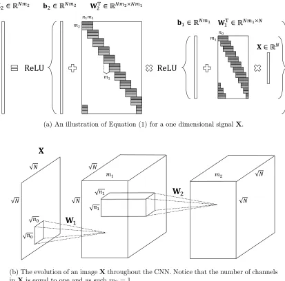
(a) An illustration of Equation (1) for a one dimensional signalX.
𝑁 𝑁
𝐗
𝑚1 𝑁
𝑁
𝑛0
𝑛0
𝐖
1
𝑚2 𝑁
𝑁 𝑛1
𝑛1
𝐖
2(b) The evolution of an imageXthroughout the CNN. Notice that the number of channels in Xis equal to one and as suchm0= 1.
Figure 2: The forward pass algorithm for a one dimensional signal (a) and an image (b).
in Figure 1b. Using this observation, the above description for one dimensional signals can be extended to images, with the exception that now every Circulant matrix is replaced by a block Circulant with Circulant blocks one.
An illustration of the forward pass algorithm is presented in Figure 2a and 2b. In Figure 2a one can observe that W2 is not a regular convolutional matrix but a stride one, since it shifts local filters by skipping m1 entries at a time. The reason for this becomes apparent once we look at Figure 2b; the convolutions of the second layer are computed by shifting the filters of W2 that are of size
√ n1×
√
Thus far, we have presented the basic structure of CNN. However, oftentimes an ad-ditional non-linear function, termed pooling, is employed on the resulting feature map ob-tained from the ReLU operator. In essence, this step summarizes each wi-dimensional spatial neighborhood from the i-th kernel map Zi by replacing it with a single value. If the neighborhoods are non-overlapping, for example, this results in the down-sampling of the feature map by a factor of wi. The most widely used variant of the above is the max pooling (Krizhevsky et al., 2012; Simonyan and Zisserman, 2014), which picks the maximal value of each neighborhood. In (Springenberg et al., 2014) it was shown that this operator can be replaced by a convolutional layer with increased stride without loss in performance in several image classification tasks. Moreover, the current state-of-the-art in image recog-nition is obtained by the residual network (He et al., 2015), which does not employ any pooling steps (except for a single layer). As such, we defer the analysis of this operator to a follow-up work.
In the context of classification, for example, the output of the last layer is fed into a simple classifier that attempts to predict the label of the input signalX, denoted byh(X). Given a set of signals {Xj}j, the task of learning the parameters of the CNN – including the filters {Wi}Ki=1, the biases {bi}Ki=1 and the parameters of the classifier U – can be formulated as the following minimization problem
min {Wi}Ki=1,{bi}Ki=1,U
X
j
`h(Xj),U, f Xj,{Wi}Ki=1,{bi}Ki=1
. (2)
This optimization task seeks for the set of parameters that minimize the mean of the loss function `, representing the price incurred when classifying the signal X incorrectly. The input for`is the true labelh(X) and the one estimated by employing the classifier defined by U on the final layer of the CNN given by f X,{Wi}Ki=1,{bi}Ki=1
. Similarly one can tackle various other problems, e.g. regression or prediction.
In the remainder of this work we shall focus on the feature extraction process and assume that the parameters of the CNN model are pre-trained and fixed. These, for example, could have been obtained by minimizing the above objective via the backpropagation algorithm and the stochastic gradient descent, as in the VGG network (Simonyan and Zisserman, 2014).
2.2 Sparse-Land
This section presents an overview of the Sparse-Land model and its many extensions. We start with the traditional sparse representation and the core problem it aims to solve, and then proceed to its nonnegative variant. Next, we continue to the dictionary learning task both in the unsupervised and supervised cases. Finally, we describe the recent CSC model, which will lead us in the next section to the proposal of the ML-CSC model. This, in turn, will naturally connect the realm of sparsity to that of the CNN.
2.2.1 Sparse Representation
In the sparse representation model one assumes a signal X ∈ RN can be described as a
multiplication of a matrixD∈RN×M, also called a dictionary, by a sparse vectorΓ∈
Equally, the signal X can be seen as a linear combination of a few columns from the dictionary D, coined atoms.
For a fixed dictionary, given a signalX, the task of recovering its sparsest representation Γis called sparse coding, or simply pursuit, and it attempts to solve the following problem (Donoho and Elad, 2003; Tropp, 2004; Elad, 2010):
(P0) : min
Γ kΓk0 s.t. DΓ=X, (3) where we have denoted by kΓk0 the number of non-zeros in Γ. The above has a convex relaxation in the form of the Basis-Pursuit (BP) problem (Chen et al., 2001; Donoho and Elad, 2003; Tropp, 2006), formally defined as
(P1) : min
Γ kΓk1 s.t. DΓ=X. (4) Many questions arise from the above two defined problems. For instance, given a signalX, is its sparsest representation unique? Assuming that such a unique solution exists, can it be recovered using practical algorithms such as the Orthogonal Matching Pursuit (OMP) (Chen et al., 1989; Pati et al., 1993) and the BP (Chen et al., 2001; Daubechies et al., 2004)? The answers to these questions were shown to be positive under the assumption that the number of non-zeros in the underlying representation is not too high and in particular less than1
2
1 + 1 µ(D)
(Donoho and Elad, 2003; Tropp, 2004; Donoho et al., 2006). The quantity
µ(D) is the mutual coherence of the dictionaryD, being the maximal inner product of two atoms extracted from it2. Formally, we can write
µ(D) = max i6=j |d
T i dj|.
Tighter conditions, relying on sharper characterizations of the dictionary, were also sug-gested in the literature (Candes et al., 2006; Schnass and Vandergheynst, 2007; Candes et al., 2006; Candes and Tao, 2007). However, at this point, we shall not dwell on these.
One of the simplest approaches for tackling the P0 and P1 problems is via the hard and soft thresholding algorithms, respectively. These operate by computing the inner products between the signal X and all the atoms in D and then choosing the atoms corresponding to the highest responses. This can be described as solving, for some scalarβ, the following problems:
min Γ
1
2kΓ−D TXk2
2+βkΓk0 for the P0, or
min Γ
1
2kΓ−D TXk2
2+βkΓk1, (5)
for the P1. The above are simple projection problems that admit a closed-form solution in the form3ofH
β(DTX) orSβ(DTX), where we have defined the hard thresholding operator
2. Hereafter, we assume that the atoms are normalized to a unit`2 norm.
Hβ(·) by
Hβ(z) =
z, z <−β
0, −β ≤z≤β z, β < z,
and the soft thresholding operatorSβ(·) by
Sβ(z) =
z+β, z <−β
0, −β ≤z≤β z−β, β < z.
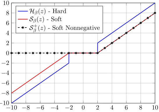
Both of the above, depicted in Figure 3, nullify small entries and thus promote a sparse solution. However, while the hard thresholding operator does not modify large coefficients (in absolute value), the soft thresholding does, by contracting these to zero. This inherent limitation of the soft version will appear later on in our theoretical analysis.
As for the theoretical guarantees for the success of the simple thresholding algorithms; these depend on the properties of D and on the ratio between the minimal and maximal coefficients in absolute value in Γ, and thus are weaker when compared to those found for OMP and BP (Donoho and Elad, 2003; Tropp, 2004; Donoho et al., 2006). Still, under some conditions, both algorithms are guaranteed to find the true support of Γ along with an approximation of its true coefficients. Moreover, a better estimation of these can be obtained by projecting the input signal onto the atoms corresponding to the found support (indices of the non-zero entries) by solving a Least-Squares problem. This step, termed debiasing (Elad, 2010), results in a more accurate identification of the non-zero values.
2.2.2 Nonnegative Sparse Coding
The nonnegative sparse representation model assumes a signal can be decomposed into a multiplication of a dictionary and anonnegative sparse vector. A natural question arising from this is whether such a modification to the original Sparse-Land model affects its ex-pressiveness. To address this, we hereby provide a simple reduction from the original sparse representation to the nonnegative one.
Consider a signal X=DΓ, where the signs of the entries inΓ are unrestricted. Notice that this can be equally written as
X=DΓP + (−D)(−ΓN),
where we have split the vector Γ to its positive coefficients, ΓP, and its negative ones,
ΓN. Since the coefficients in ΓP and −ΓN are all positive, one can thus assume the sig-nal X admits a non-negative sparse representation over the dictionary [D,−D] with the vector [ΓP,−ΓN]T. Thus, restricting the coefficients in the sparsity inspired model to be nonnegative does not change its expressiveness.
Similar to the original model, in the nonnegative case, one could solve the associated pursuit problem by employing a soft thresholding algorithm. However, in this case a con-straint must be added to the optimization problem in Equation (5), forcing the outcome to be positive, i.e.,
min Γ
1
2kΓ−D TXk2
−10 −8 −6 −4 −2 0 2 4 6 8 10
−10
−8
−6
−4
−2 0 2 4 6 8 10
Hβ(z) - Hard
Sβ(z) - Soft
Sβ+(z) - Soft Nonnegative
Figure 3: The thresholding operators for a constantβ= 2.
Since the above is a simple projection problem (onto the `1 ball constrained to positive entries), it admits a closed-form solution Sβ+(DTX), where we have defined the soft non-negative thresholding operatorSβ+(·) as
Sβ+(z) =
(
0, z≤β z−β, β < z.
Remarkably, the above function satisfies
Sβ+(z) = max(z−β,0) = ReLU(z−β).
In other words, the ReLU and the soft nonnegative thresholding operator are equal, a fact that will prove to be important later in our work. We should note that a similar conclusion was reached in (Fawzi et al., 2015). To summarize this discussion, we depict in Figure 3 the hard, soft, and nonnegative soft thresholding operators.
2.2.3 Unsupervised and Task Driven Dictionary Learning
The task of learning a dictionary for representing a set of signals{Xj}jcan be formulated as follows
min D,{Γj}
j
X
j
kXj−DΓjk22+ξkΓjk0.
The above formulation is an unsupervised learning procedure, and it was later extended to a supervised setting. In this context, given a set of signals{Xj}j, one attempts to predict their corresponding labels {h(Xj)}j. A common approach for tackling this is first solving a pursuit problem for each signalXj over a dictionary D, resulting in
Γ?(Xj,D) = arg min Γ
kΓk0 s.t. DΓ=Xj,
and then feeding these sparse representations into a simple classifier, defined by the param-eters U. The task of learning jointly the dictionary D and the classifier U was addressed in (Mairal et al., 2012), where the following optimization problem was proposed
min D,U
X
j
`h(Xj),U,Γ?(Xj,D)
.
The loss function ` in the above objective penalizes the estimated label if it is different from the true h(Xj), similar to what we have seen in Section 2.1. The above formulation contains in it the unsupervised option as a special case, in which U is of no importance, and the loss function is the representation error P
jkXj−DΓ?jk22.
Double sparsity – first proposed in (Rubinstein et al., 2010) and later employed in (Su-lam et al., 2016) – attempts to benefit from both the computational efficiency of analytically defined matrices, and the adaptability of data driven dictionaries. In this model, one as-sumes the dictionaryD can be factorized into a multiplication of two matrices,D1 andD2, where D1 is an analytic dictionary with fast implementation, and D2 is a trained sparse one. As a result, the signalX can be represented as
X=DΓ2 =D1D2Γ2, whereΓ2 is sparse.
We propose a different interpretation for the above, which is unrelated to practical aspects. Since both the matrix D2 and the vector Γ2 are sparse, one would expect their multiplicationΓ1=D2Γ2to be sparse as well. As such, the double sparsity model implicitly assumes that the signalX can be decomposed into a multiplication of a dictionaryD1 and sparse vectorΓ1, which in turn can also be decomposed similarly via Γ1=D2Γ2.
2.2.4 Convolutional Sparse Coding Model
Due to the computational constraints entailed when deploying trained dictionaries, this approach seems valid only for treatment of low-dimensional signals. Indeed, the sparse representation model is traditionally used for modeling local patches extracted from a global signal. An alternative, which was recently proposed, is the CSC model that attempts to represent the whole signal X∈RN as a multiplication of a global convolutional dictionary
𝑚
=
𝛀
∈ ℝ
𝑛× 2𝑛−1 𝑚𝐱i ∈ ℝ𝑛 𝛄i ∈ ℝ2𝑛−1 𝑚
𝑚
𝑛
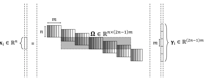
Figure 4: Thei-th patch xi of the global system X=DΓ, given by xi=Ωγi.
shifting a local matrix of sizen×min all possible positions, resulting in the same structure as the one shown in Figure 1a.
In the convolutional model, the classical theoretical guarantees (we are referring to results reported in (Chen et al., 2001; Donoho and Elad, 2003; Tropp, 2006)) for the P0 problem, defined in Equation (3), are very pessimistic. In particular, the condition for the uniqueness of the underlying solution and the requirement for the success of the sparse coding algorithms depend on the global number of non-zeros being less than 1
2
1 + 1 µ(D)
. Following the Welch bound (Welch, 1974), this expression was shown in (Papyan et al., 2016a) to be impractical, allowing the global number of non-zeros inΓto be extremely low. In order to provide a better theoretical understanding of this model, which exploits the inherent structure of the convolutional dictionary, a recent work (Papyan et al., 2016a) suggested to measure the sparsity of Γ in a localized manner. More concretely, consider thei-thn-dimensional patch of the global systemX=DΓ, given byxi =Ωγi. The stripe-dictionary Ω, which is of size n×(2n−1)m, is obtained by extracting thei-th patch from the global dictionary D and discarding all the zero columns from it. The stripe vector γi is the corresponding sparse representation of length (2n−1)m, containing all coefficients of atoms contributing to xi. This relation is illustrated in Figure 4. Notably, the choice of a convolutional dictionary results in signals such that every patch of length nextracted from them can be sparsely represented using a single shift-invariant local dictionary Ω– a common assumption usually employed in signal and image processing.
Following the above construction, the`0,∞norm of the global sparse vectorΓis defined to be the maximal number of non-zeros in a stripe of length (2n−1)m extracted from it. Formally,
kΓkS
0,∞= max i kγik0,
where the letters emphasizes that the `0,∞ norm is computed by sweeping over all stripes. Given a signal X, finding its sparest representation Γ in the `0,∞ sense is equal to the following optimization problem:
(P0,∞) : min Γ kΓk
S
Intuitively, this seeks for a global vector Γ that can represent sparsely every patch in the signal Xusing the dictionary Ω. The advantage of the above problem over the traditional P0 becomes apparent as we move to consider its theoretical aspects. Assuming that the
number of non-zeros per stripe (and not globally) in Γ is less than 121 +µ(D)1 , in (Papyan et al., 2016a) it was proven that the solution for the P0,∞ problem is unique. Furthermore, classical pursuit methods, originally tackling the P0 problem, are guaranteed to find this representation.
When modeling natural signals, due to measurement noise as well as model deviations, one can not impose a perfect reconstruction such asX=DΓon the signalX. Instead, one assumesY =X+E=DΓ+E, where E is, for example, an `2-bounded error vector. To address this, the work reported in (Papyan et al., 2016b) considered the extension of the P0,∞ problem to the PE0,∞ one, formally defined as
(PE0,∞) : min Γ kΓk
S
0,∞ s.t. kY−DΓk22 ≤E2.
Similar to the P0,∞ problem, this was also analyzed theoretically, shedding light on the theoretical aspects of the convolutional model in the presence of noise. In particular, a stability claim for the PE0,∞ problem and guarantees for the success of both the OMP and the BP were provided. Similar to the noiseless case, these assumed that the number of non-zeros per stripe is low.
3. From Atoms to Molecules: Multi-Layer Convolutional Sparse Model
Convolutional sparsity assumes an inherent structure for natural signals. Similarly, the representations themselves could also be assumed to have such a structure. In what follows, we propose a novel layered model that relies on this rationale.
The convolutional sparse model assumes a global signal X ∈ RN can be decomposed into a multiplication of a convolutional dictionary D1 ∈ RN×N m1, composed of m1 local filters of lengthn0, and a sparse vector Γ1 ∈RN m1. Herein, we extend this by proposing a
similar factorization of the vector Γ1, which can be perceived as an N-dimensional global signal with m1 channels. In particular, we assume Γ1 = D2Γ2, where D2 ∈ RN m1×N m2
is a stride convolutional dictionary (skipping m1 entries at a time) and Γ2 ∈ RN m2 is a
sparse representation. We denote the number of unique filters constructing D2 by m2 and their corresponding length by n1m1. Due to the multi-layer nature of this model and the imposed convolutional structure, we name this the ML-CSC model.
Intuitively, X = D1Γ1 assumes that the signal X is a superposition of atoms taken fromD1. While equationX=D1D2Γ2 views the signal as a superposition of more complex entities taken from the dictionaryD1D2, which we coin molecules.
𝑚1 𝑛0
𝐃1∈ ℝ𝑁×𝑁𝑚1 𝚪
1∈ ℝ𝑁𝑚1
𝐗 ∈ ℝ𝑁
𝚪1∈ ℝ𝑁𝑚1
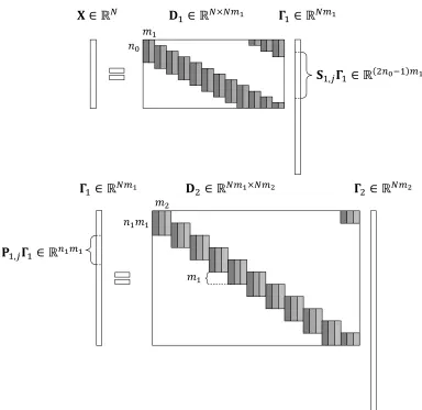
𝑛1𝑚1 𝑚2
𝐒1,𝑗𝚪1∈ ℝ 2𝑛0−1 𝑚1
𝐏1,𝑗𝚪1∈ ℝ𝑛1𝑚1
𝐃2∈ ℝ𝑁𝑚1×𝑁𝑚2 𝚪
2 ∈ ℝ𝑁𝑚2
𝑚1
Figure 5: An instanceX=D1Γ1 =D1D2Γ2 of the ML-CSC model. Notice thatΓ1 is built of both stripes S1,jΓ1 and patchesP1,jΓ1.
Under the above construction the sparse vector Γ1 has two roles. In the context of the system of equations X = D1Γ1, it is the convolutional sparse representation of the signal X over the dictionary D1. As such, the vector Γ1 is composed from (2n0 −1)m1 -dimensional stripes, S1,jΓ1, where Si,j is the operator that extracts the j-th stripe from
Γi. From another point of view, Γ1 is in itself a signal that admits a sparse representation
Γ1 =D2Γ2. Denoting by Pi,j the operator that extracts thej-th patch fromΓi, the signal
Definition 1 For a global signal X, a set of convolutional dictionaries {Di}Ki=1, and a vector λ, define the deep coding problem DCPλ as:
(DCPλ) : find {Γi}Ki=1 s.t. X=D1Γ1, kΓ1kS0,∞≤λ1
Γ1 =D2Γ2, kΓ2kS0,∞≤λ2 ..
. ...
ΓK−1 =DKΓK, kΓKkS0,∞≤λK, where the scalarλi is the i-th entry of λ.
Denoting Γ0 to be the signalX, the DCPλ can be rewritten compactly as
(DCPλ) : find {Γi}Ki=1 s.t. Γi−1 =DiΓi, kΓikS0,∞≤λi, ∀1≤i≤K. Intuitively, given a signal X, this problem seeks for a set of representations, {Γi}Ki=1, such that each one is locally sparse. As we shall see next, the above can be easily solved using simple algorithms that also enjoy from theoretical justifications. Next, we extend the DCPλ
problem to a noisy regime.
Definition 2 For a global signalY, a set of convolutional dictionaries{Di}Ki=1, and vectors λ and E, define the deep coding problem DCPλE as:
(DCPλE) : find {Γi}Ki=1 s.t. kY−D1Γ1k2 ≤ E0, kΓ1kS0,∞≤λ1
kΓ1−D2Γ2k2 ≤ E1, kΓ2kS0,∞≤λ2 ..
. ...
kΓK−1−DKΓKk2 ≤ EK−1, kΓKkS0,∞≤λK, where the scalars λi andEi are the i-th entry ofλ and E, respectively.
We now move to the task of learning the model parameters. Denote by DCP?
λ(X,{Di}Ki=1) the representation ΓK obtained by solving the DCP problem (Definition 1, i.e., noiseless) for the signal X and the set of dictionaries {Di}Ki=1. Relying on this, we now extend the dictionary learning problem, as presented in Section 2.2.3, to the multi-layer convolutional sparse representation setting.
Definition 3 For a set of global signals {Xj}j, their corresponding labels {h(Xj)}j, a loss function`, and a vector λ, define the deep learning problem DLPλ as:
(DLPλ) : min
{Di}Ki=1,U
X
j
`
h(Xj),U,DCPλ?(Xj,{Di}Ki=1)
.
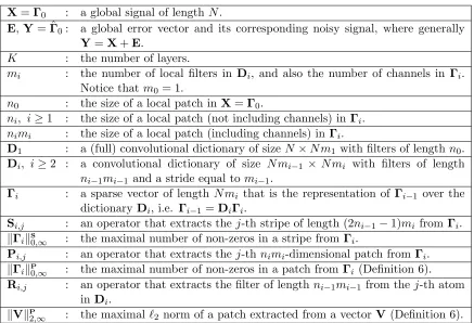
X=Γ0 : a global signal of length N.
E,Y= ˆΓ0: a global error vector and its corresponding noisy signal, where generally
Y =X+E.
K : the number of layers.
mi : the number of local filters in Di, and also the number of channels in Γi. Notice that m0 = 1.
n0 : the size of a local patch inX=Γ0.
ni, i≥1 : the size of a local patch (not including channels) in Γi.
nimi : the size of a local patch (including channels) in Γi.
D1 : a (full) convolutional dictionary of size N×N m1 with filters of lengthn0.
Di, i≥2 : a convolutional dictionary of size N mi−1 × N mi with filters of length
ni−1mi−1 and a stride equal tomi−1.
Γi : a sparse vector of length N mi that is the representation of Γi−1 over the dictionary Di, i.e. Γi−1 =DiΓi.
Si,j : an operator that extracts the j-th stripe of length (2ni−1−1)mi from Γi.
kΓikS0,∞ : the maximal number of non-zeros in a stripe from Γi.
Pi,j : an operator that extracts the j-thnimi-dimensional patch from Γi.
kΓikP0,∞ : the maximal number of non-zeros in a patch from Γi (Definition 6).
Ri,j : an operator that extracts the filter of lengthni−1mi−1 from thej-th atom inDi.
kVkP
2,∞ : the maximal`2 norm of a patch extracted from a vectorV (Definition 6). Table 1: Summary of notations used throughout the paper.
4. Layered Thresholding: The Crux of the Matter
Consider the ML-CSC model defined by the set of dictionaries {Di}Ki=1. Assume we are given a signal
X=D1Γ1
Γ1 =D2Γ2 .. .
ΓK−1 =DKΓK,
and our goal is to find its underlying representations, {Γi}Ki=1. Tackling this problem by recovering all the vectors at once might be computationally and conceptually challenging; therefore, we propose thelayered thresholding algorithmthat gradually computes the sparse vectors one at a time across the different layers. Denoting by Pβ(·) a sparsifying operator that is equal toHβ(·) in the hard thresholding case andSβ(·) in the soft one; we commence by computing ˆΓ1 =Pβ1(D
T
1X), which is an approximation ofΓ1. Next, by applying another thresholding algorithm, however this time on ˆΓ1, an approximation ofΓ2 is obtained, ˆΓ2=
Pβ2(DT2Γˆ1). This process, which is iterated until the last representation ˆΓK is acquired, is summarized in Algorithm 1.
Algorithm 1 The layered thresholding algorithm. Input:
X – a signal.
{Di}Ki=1 – convolutional dictionaries.
P ∈ {H,S,S+}– a thresholding operator.
{βi}K
i=1 – thresholds.
Output:
A set of representations {Γˆi}Ki=1.
Process:
1: Γˆ0 ←X
2: fori= 1 :K do
3: Γˆi← Pβi(D T i Γˆi−1) 4: end for
previously described in Section 2.2.1, assuming some conditions are met, the result of the thresholding algorithm, ˆΓ1, is guaranteed to have the correct support. In order to obtain the vectorΓ1 itself, one should project the signalXonto this obtained support, by solving a Least-Squares problem. For reasons that will become clear shortly, we choose not to employ this step in the layered thresholding algorithm. Despite this algorithm failing in recovering the exact representations in the noiseless setting, as we shall see in Section 5, the estimated sparse vectors and the true ones are close – indicating the stability of this simple algorithm. Thus far, we have assumed a noiseless setting. However, the same layered thresholding algorithm could be employed for the recovery of the representations of a noisy signal Y= X+E, with the exception that the threshold constants, {βi}Ki=1, would be different and proportional to the noise level.
Assuming two layers for simplicity, Algorithm 1 can be summarized in the following equation
ˆ
Γ2=Pβ2
DT2Pβ1 DT1X
.
Comparing the above with Equation (1), given by
f(X,{Wi}i=12 ,{bi}2i=1) = ReLU
WT2 ReLU WT1X+b1
+b2
,
one can notice a striking similarity between the two. Moreover, by replacingPβ(·) with the soft nonnegative thresholding, Sβ+(·), we obtain that the aforementioned pursuit and the forward pass of the CNN are equal! Notice that we are relying here on the discussion of Section 2.2.2, where we have shown that the ReLU and the soft nonnegative thresholding are equal4.
Recall the optimization problem of the training stage of the CNN as shown in Equation (2), given by
min {Wi}Ki=1,{bi}Ki=1,U
X
j
`h(Xj),U, f Xj,{Wi}Ki=1,{bi}Ki=1
,
and its parallel in the ML-CSC model, the DLPλ problem, defined by
min {Di}Ki=1,U
X
j
`
h(Xj),U,DCPλ?(Xj,{Di}Ki=1)
.
Notice the remarkable similarity between both objectives, the only difference being in the feature vector on which the classification is done; in the CNN this is the output of the forward pass algorithm, given byf Xj,{Wi}Ki=1,{bi}Ki=1
, while in the sparsity case this is the result of the DCPλproblem. In light of the discussion above, the solution for the DCPλ
problem can be approximated using the layered thresholding algorithm, which is in turn equal to the forward pass of the CNN. We can therefore conclude that the problems solved by the training stage of the CNN and the DLPλare tightly connected, and in fact are equal
once the solution for the DLPλ is approximated via the layered thresholding algorithm
(hence the name DLPλ).
5. Theoretical Study
Thus far, we have defined the ML-CSC model and its corresponding pursuits – the DCPλ
and DCPλE problems. We have proposed a method to tackle them, coined the layered thresh-olding algorithm, which was shown to be equivalent to the forward pass of the CNN. Relying on this, we conclude that the proposed ML-CSC is the global Bayesian model implicitly imposed on the signal X when deploying the forward pass algorithm. Put differently, the ML-CSC answers the question of who are the signals belonging to the model behind the CNN. Having established the importance of our model, we now proceed to its theoretical analysis.
We should emphasize that the following study does not assume any specific form on the network’s parameters, apart from a broad coherence property (as will be shown hereafter). This is in contrast to the work of (Bruna and Mallat, 2013) that assumes that the filters are Wavelets, or the analysis in (Giryes et al., 2015) that considers random weights.
5.1 Uniqueness of the DCPλ Problem
Consider a signalXadmitting a multi-layer convolutional sparse representation defined by the sets {Di}Ki=1 and {λi}Ki=1. Can another set of sparse vectors represent the signal X? In other words, can we guarantee that, under some conditions, the set {Γi}Ki=1 is a unique solution to the DCPλ problem? In the following theorem we provide an answer to this
Theorem 4 (Uniqueness via the mutual coherence): Consider a signal X satisfying the DCPλ model,
X=D1Γ1
Γ1 =D2Γ2 .. .
ΓK−1 =DKΓK,
where {Di}Ki=1 is a set of convolutional dictionaries and{µ(Di)}Ki=1 are their corresponding mutual coherences. If
∀ 1≤i≤K kΓikS0,∞< 1 2
1 + 1
µ(Di)
,
then the set{Γi}Ki=1 is the unique solution to the DCPλ problem, assuming that the
thresh-olds{λi}Ki=1 are chosen to satisfy
∀1≤i≤K kΓikS0,∞≤λi< 1 2
1 + 1
µ(Di)
.
The proof for the above theorem is given in Appendix A. In what follows, we present its importance in the context of CNN. Assume a signalXis fed into a network, resulting in a set of activation values across the different layers. These, in the realm of sparsity, correspond to the set of sparse representations {Γi}Ki=1, which according to the above theorem are in fact unique representations of the signalX.
One might ponder at this point whether there exists an algorithm for obtaining the unique solution guaranteed in this subsection for the DCPλ problem. As previously
men-tioned, the layered thresholding algorithm is incapable of finding the exact representations,
{Γi}Ki=1, due to the lack of a Least-Squares step after each layer. One should not despair, however, as we shall see in a following section an alternative algorithm, which manages to overcome this hurdle.
5.2 Global Stability of the DCPλE Problem
Consider an instance signalXbelonging to the ML-CSC model, defined by the sets{Di}Ki=1 and{λi}Ki=1. AssumeXis contaminated by a noise vectorE, generating the perturbed signal
Y = X+E. Suppose we solve the DCPλE problem and obtain a set of solutions {Γˆi}Ki=1. How close is every solution in this set, ˆΓi, to its corresponding true representation, Γi? In what follows, we provide a theorem addressing this question of stability, the proof of which is deferred to Appendix B.
Theorem 5 (Stability of the solution to the DCPλE problem): Suppose a signalX that has a decomposition
X=D1Γ1
Γ1=D2Γ2 .. .
is contaminated with noiseE, resulting inY=X+E. Assume we solve the DCPλE problem for E0 = kEk2 and Ei = 0 ∀1 ≤ i ≤ K, obtaining a set of solutions {Γˆi}Ki=1. If for all 1≤i≤K
kΓikS0,∞≤λi < 1 2
1 + 1
µ(Di)
,
then
kΓi−Γˆik22≤4kEk22 i
Y
j=1
1
1−(2λj −1)µ(Dj)
.
Intuitively, the above claims that as long as all the feature vectors {Γi}Ki=1 are `0,∞ -sparse, then the representations obtained by solving the DCPλE problem must be close to the true ones. Interestingly, the obtained bound increases as a function of the depth of the layer.
Is this necessarily the true behavior of a deep network? Perhaps the answer to this resides in the choice we made above of considering the noise as adversary. A similar, yet somewhat more involved, analysis with a random noise assumption should be done, with the hope to see a better controlled noise propagation in this system. We leave this for our future work.
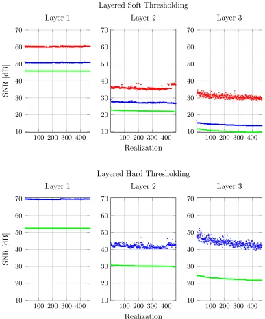
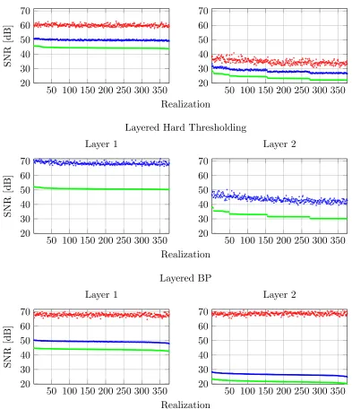
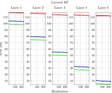
Another important remark is that the above bounds the absolute error between the estimated and the true representation. In practice, however, the relative error is of more importance. This is measured in terms of the signal to noise ratio (SNR), which we shall define in Section 8.
Having established the stability of the DCPλE problem, we now turn to the stability of the algorithms attempting to solve it, the chief one being the forward pass of CNN.
5.3 Stability of the Layered Hard Thresholding
Consider a signal X that admits a multi-layer convolutional sparse representation, which is defined by the sets {Di}Ki=1 and {λi}Ki=1. Assume we run the layered hard thresholding algorithm on X, obtaining the sparse vectors {Γˆi}Ki=1. Under certain conditions, can we guarantee that the estimate ˆΓi recovers the true support of Γi? or that the norm of the difference between the two is bounded? Assume X is contaminated with a noise vector E, resulting in the measurement Y =X+E. Assume further that this signal is then fed to the layered thresholding algorithm, resulting in another set of representations. How do the answers to the above questions change? To tackle these, we commence by presenting a stability claim for the simple hard thresholding algorithm, relying on the `0,∞ norm. We should note that the analysis conducted in this subsection is for the noisy scenario, and the results for the noiseless case are simply obtained by setting the noise level to zero.
Next, we present a localized `2 and `0 measure of a global vector that will prove to be useful in the following analysis.
Definition 6 Define the k · kP
2,∞ andk · kP0,∞ norm of Γi to be
kΓikP2,∞= max
and
kΓikP0,∞= max
j kPi,jΓik0,
respectively. The operator Pi,j extracts the j-th patch of length nimi from the i-th sparse vector Γi.
In the above definition, the letter p emphasizes that the norms are computed by sweeping over all patches, rather than stripes. Recall that we have definedm0= 1, since the number of channels in the input signalX=Γ0 is equal to one.
Given Y = X+E = D1Γ1 +E, the first stage of the layered hard thresholding algo-rithm attempts to recover the representationΓ1. Intuitively, assuming that the underlying representation Γ1 is `0,∞-sparse, and that the energy of the noise E is `2,∞-bounded; we would expect that the simple hard thresholding algorithm would succeed in recovering a solution ˆΓ1, which is both close to Γ1 and has its support. We now present such a claim, the proof of which is found in Appendix C.
Lemma 7 (Stable recovery of hard thresholding in the presence of noise): Suppose a clean signal X has a convolutional sparse representation D1Γ1, and that it is contaminated with noise E to create the signal Y = X+E, such that kEkP
2,∞ ≤ 0. Denote by |Γmin1 | and
|Γmax
1 |the lowest and highest entries in absolute value in Γ1, respectively. Denote further by ˆ
Γ1 the solution obtained by running the hard thresholding algorithm on Y with a constant
β1, i.e. Γˆ1=Hβ1(D
T
1Y). Assuming that a) kΓ1kS0,∞< 12
1 + 1 µ(D1)
|Γmin
1 |
|Γmax
1 |
− 1
µ(D1)
0
|Γmax
1 |; and
b) The threshold β1 is chosen according to Equation(14) (see below), then the following must hold:
1. The support of the solution Γˆ1 is equal to that of Γ1; and 2. kΓ1−Γˆ1kP2,∞≤
q
kΓ1kP0,∞
0+µ(D1) kΓ1kS0,∞−1
|Γmax 1 |
.
Notice that by plugging0 = 0 the above theorem covers the noiseless scenario. Notably, even in such a case, we obtain a deviation from the true representation due to the lack of a Least-Squares step.
We suspect that, both in the noiseless and the noisy case, the obtained bound might be improved, based on the following observation. Given an `2,∞-norm bounded noise, the above proof first quantifies the deviation between the true representation and the estimated one in terms of the `∞ norm, and only then translates the latter into the `2,∞ sense. A direct analysis going from an `2,∞ input error to an `2,∞ output deviation (bypassing the
`∞ norm) might lead to smaller deviations. We leave this for future work.
Theorem 8 (Stability of layered hard thresholding in the presence of noise): Suppose a clean signal X has a decomposition
X=D1Γ1
Γ1 =D2Γ2 .. .
ΓK−1 =DKΓK,
and that it is contaminated with noiseEto create the signalY=X+E, such thatkEkP
2,∞≤
0. Denote by|Γmini |and|Γmaxi |the lowest and highest entries in absolute value in the vector
Γi, respectively. Let {Γˆi}Ki=1 be the set of solutions obtained by running the layered hard thresholding algorithm with thresholds {βi}Ki=1, i.e. Γˆi = Hβi(D
T
iΓˆi−1) where Γˆ0 = Y. Assuming that ∀ 1≤i≤K
a) kΓikS0,∞< 12
1 + 1 µ(Di)
|Γmin
i | |Γmax
i |
− 1
µ(Di) i−1
|Γmax
i |; and b) The threshold βi is chosen according to Equation(19),
then5
1. The support of the solution Γˆi is equal to that of Γi; and
2. kΓi−ΓˆikP2,∞≤i, where i=
q
kΓikP0,∞
i−1+µ(Di) kΓikS0,∞−1
|Γmax i |
.
The proof for the above is given in Appendix D. We now turn to an analogous theorem for the forward pass of the CNN, prior to discussing the surprising implications of these theorems.
5.4 Stability of the Forward Pass (Layered Soft Thresholding)
In light of the discussion in Section 4, the equivalence between the layered thresholding algorithm and the forward pass of the CNN is achieved assuming that the operator em-ployed is the nonnegative soft thresholding Sβ+(·). However, thus far, we have analyzed the closely related hard version Hβ(·) instead. In what follows, we show how the stability theorem presented in the previous subsection can be modified to the soft version,Sβ(·). For simplicity, and in order to stay in line with the vast sparse representation theory, herein we choose not to assume the nonnegative assumption. This implies that we are proposing a slightly different CNN architecture in which the ReLU function is two sided (Kavukcuoglu et al., 2010). We now move to the stable recovery of the soft thresholding algorithm.
5. Recall thatkΓikP2,∞is defined to be the maximal`2 norm of a patch extract fromΓi. The size of this
patch is defined according to the dictionaryDi+1. However, the last sparse vectorΓK does not have a
corresponding dictionaryDK+1. As such, the size of a patch in ΓK can be chosen arbitrarily. Where
the choice of the size directly affects the bound on the difference,i, due to the term
q
Lemma 9 (Stable recovery of soft thresholding in the presence of noise): Suppose a clean signal X has a convolutional sparse representation D1Γ1, and that it is contaminated with noise E to create the signal Y = X+E, such that kEkP
2,∞ ≤ 0. Denote by |Γmin1 | and
|Γmax
1 | the lowest and highest entries in absolute value in Γ1, respectively. Denote further by Γˆ1 the solution obtained by running the soft thresholding algorithm onY with a constant
β1, i.e. Γˆ1=Sβ1(D
T
1Y). Assuming that a) kΓ1kS0,∞< 12
1 + 1 µ(D1)
|Γmin 1 | |Γmax 1 | − 1
µ(D1)
0
|Γmax
1 |; and
b) The threshold β1 is chosen according to Equation(14), then the following must hold:
1. The support of the solution Γˆ1 is equal to that of Γ1; and 2. kΓ1−Γˆ1kP2,∞≤
q
kΓ1kP0,∞
0+µ(D1) kΓ1kS0,∞−1
|Γmax 1 |+β1
.
Armed with the above lemma, which is proven in Appendix E, we now proceed to the stability of the forward pass of the CNN.
Theorem 10 (Stability of the forward pass (layered soft thresholding algorithm) in the presence of noise): Suppose a clean signal X has a decomposition
X=D1Γ1
Γ1 =D2Γ2 .. .
ΓK−1 =DKΓK,
and that it is contaminated with noiseEto create the signalY=X+E, such thatkEkP
2,∞≤
0. Denote by |Γmini | and |Γmaxi | the lowest and highest entries in absolute value in the vector Γi, respectively. Let {Γˆi}Ki=1 be the set of solutions obtained by running the layered soft thresholding algorithm with thresholds {βi}K
i=1, i.e. Γˆi =Sβi(D T
i Γˆi−1) where Γˆ0 =Y. Assuming that ∀ 1≤i≤K
a) kΓikS0,∞< 12
1 + 1 µ(Di)
|Γmin i | |Γmax i | − 1
µ(Di) i−1
|Γmax
i |; and
b) The threshold βi is chosen according to Equation(19) (with the i defined below),
then
1. The support of the solution Γˆi is equal to that of Γi; and
2. kΓi−ΓˆikP2,∞≤i, where i=
q
kΓikP0,∞
i−1+µ(Di) kΓikS0,∞−1
|Γmax i |+βi
The proof for the above is omitted since it is tantamount to that of Theorem 8. As one can see, the layered soft thresholding algorithm is in fact inferior to its hard variant due to the added constant of βi in the local error level, i. This results in a more strict assumption on the `0,∞ norm of the various representations and also augments the bound on the distance between the true sparse vector and the one recovered. Following this observation, a natural question arises; why does the deep learning community employ the ReLU, which corresponds to a soft nonnegative thresholding operator instead of another nonlinearity that is more similar to its hard counterpart? One possible explanation could be that the filter training stage of the CNN becomes harder when the ReLU is replaced with a non-convex alternative, which also has discontinuities, such as the hard thresholding operator.
The above theorem guarantees that the distances between the original representations and the ones obtained from the CNN are bounded. Even if we set 0 = 0, the recovered activations deviate from the true ones, simply because the layered thresholding algorithm does not do a perfect job, even on a noiseless signal. When the signal is noisy, these deviations are strengthened, but still in a controlled way.
This, by itself, might not be surprising. After all, the CNN is a deterministic system of linear operations (convolutions), followed by simple non-linearities that are non-expanding. If we feed a slightly perturbed signal to such a system, it is clear that the activations all along the network will be perturbed as well with a bounded effect. However, the above theorem shows far more than that. There are, in fact, two types of stabilities, the trivial one that considers the sensitivity of the whole feed-forward network to perturbations in its input, and the more intricate one that shows that this system enables a rather accurate recovery of thegenerating representations. The second option is the stability we prove here.
5.5 Guarantees for Fully Connected Networks
One should note that the convolutional structure imposed on the dictionaries in our model could be removed, and the theoretical guarantees we have provided above would still hold. The reason being is that the unconstrained dictionary can be regarded as a convolutional one, constructed from a single shift of a local matrix with no circular boundary. In the context of CNN, this is analogous to a fully connected layer. As such, the theoretical analysis provided here sheds light on both convolutional and fully connected networks. A different point of view on the same matter can also be proposed; fully connected layers can be viewed as convolutional ones with filters that cover their entire input (Long et al., 2015).
5.6 Worst-Case Analysis
Sharper bounds, relying on stronger characterizations of the dictionary, result in signif-icantly harder analysis. One example for a different characterization is that of the average mutual coherence – defined to be the average correlation in absolute value between two distinct atoms taken from the dictionary (instead of the highest correlation, as measured by the original mutual coherence). From a theoretical point of view, this measure was shown to lead to better theoretical guarantees in classic sparse theory (Bajwa et al., 2012). In ad-dition, from a practical point of view, it was proven beneficial penalizing over this quantity in compressed sensing applications (Elad, 2007).
Our analysis did not rely on the average mutual coherence, but rather on the maximal coherence. Still, the two are closely related, and following the discussion above we believe that this might predict better the performance of CNN in practice. Interestingly, the work of (Shang, 2015) measured the average mutual coherences of the different layers in the “all-conv” network, which was trained on the ImageNet dataset (Springenberg et al., 2014). The authors found that most layers have a low average mutual coherence.
6. Layered Basis Pursuit
The stability analysis presented above unveils two significant limitations of the forward pass of the CNN. First, this algorithm is incapable of recovering the unique solution for the DCPλ problem, the existence of which is guaranteed from Theorem 4. This acts against
our expectations, since in the traditional sparsity inspired model it is a well known fact that such a unique representation can be retrieved, assuming certain conditions are met.
The second issue is with the condition for the successful recovery of the true support. The `0,∞ norm of the true solution, Γi, is required to be less than an expression that depends on the term|Γmin
i |/|Γmaxi |. The dependence on this ratio is a direct consequence of the forward pass algorithm relying on the simple thresholding operator that is known for having such a theoretical limitation6. However, alternative pursuits whose success would not depend on this ratio could be proposed, as indeed was done in the Sparse-Land model; resulting in both theoretical and practical benefits.
A solution for the first problem, already presented throughout this work, is a two-stage approach. First, run the thresholding operator in order to recover the correct support. Then, once the atoms are chosen, their corresponding coefficients can be obtained by solving a linear system of equations. In addition to retrieving the true representation in the noiseless case, this step can also be beneficial in the noisy scenario, resulting in a solution closer to the underlying one. However, since no such step exists in current CNN architectures, we refrain from further analyzing its theoretical implications.
Next, we present an alternative to the layered soft thresholding algorithm, which will tackle both of the aforementioned problems. Recall that the result of the soft thresholding is a simple approximation of the solution for the P1 problem, previously defined in Equation (4). In every layer, instead of applying a simple thresholding operator that estimates the sparse vector by computing ˆΓi =Sβi(D
T
i Γˆi−1); we propose to tackle the full pursuit, i.e. to
minimize
ˆ
Γi= arg min Γi
kΓik1 s.t. ˆΓi−1 =DiΓi. (7) Notice that one could readily obtain the nonnegative sparse coding problem by simply adding an extra constraint in the above equation, forcing the coefficients in Γi to be non-negative. More generally, Equation (7) can be written in its Lagrangian formulation
ˆ
Γi= arg min Γi
ξikΓik1+ 1
2kDiΓi−Γˆi−1k 2
2, (8)
where the constant ξi is proportional to the noise level and should tend to zero in the noiseless scenario. We name the above thelayered basis pursuit(BP) algorithm. In practice, one possible method for solving it is the iterative soft thresholding (IST). Formally, this obtains the minimizer of Equation (8) by repeating the following recursive formula
ˆ Γti =Sξ
i/ci
ˆ
Γt−1i + 1
ci
DTi Γˆi−1−DiΓˆt−1i
, (9)
where ˆΓti is the estimate of Γi at iteration t. The above can be interpreted as a simple projected gradient descent algorithm, where the constant ci is inversely proportional to its step size. As a result, if ci is chosen to be large enough7, the above algorithm is guaranteed to converge to its global minimum that is the solution of (8), as was shown in (Daubechies et al., 2004). The method obtained by gradually computing the set of sparse representations, {Γi}Ki=1, via the IST is summarized in Algorithm 2 and named layered iterative soft thresholding. Notice that this algorithm coincides with the simple layered soft thresholding if it is run for a single iteration with ci = 1 and initialized with ˆΓ0i =0. This implies that the above algorithm is a natural extension to the forward pass of the CNN. Moreover, the above is similar to the approach taken in the work of deconvolutional networks (Zeiler et al., 2010), where the authors suggested to solve a sequence of BP problems across different layers of abstraction.
With respect to the computational aspects of the IST algorithm, the work of (Gregor and LeCun, 2010) proposed the LISTA method, showing how the number of iterations required by the IST to convergence can be reduced using neural networks. Later, (Giryes et al., 2016) proved the theoretical justification for this algorithm, and (Sprechmann et al., 2015) extended LISTA to other sparse and low-rank problems. Analogously, the work of (Xin et al., 2016) presented a generalization for the iterative hard thresholding (IHT), which was shown to be both theoretically and empirically superior to the original IHT.
The original motivation for the layered IST was its theoretical superiority over the forward pass algorithm – one that will be explored in detail in the next subsection. Yet more can be said about this algorithm and the CNN architecture it induces. In (Gregor and LeCun, 2010) it was shown that the IST algorithm can be formulated as a simple recurrent neural network. As such, the same can be said regarding the layered IST algorithm proposed here, with the exception that the induced recurrent network is much deeper. The reader can
7. The constantci should satisfyci>0.5λmax DTiDi
, whereλmax DTiDi
Algorithm 2 The layered iterative soft thresholding algorithm. Input:
X – a signal.
{Di}Ki=1 – convolutional dictionaries.
P ∈ {S,S+} – a soft thresholding operator.
{ξi}K
i=1 – Lagrangian parameters.
{1/ci}Ki=1 – step sizes.
{Ti}Ki=1 – number of iterations.
Output:
A set of representations {Γˆi}Ki=1.
Process:
1: Γˆ0 ←X
2: fori= 1 :K do
3: Γˆ0i ←0
4: for t= 1 :Ti do
5: Γˆti ← Pξi/ciΓˆt−1i +c1 iD
T i
ˆ
Γi−1−DiΓˆt−1i
6: end for
7: Γˆi←ΓˆTii 8: end for
therefore interpret this part of the work as a theoretical study of a special case of recurrent neural networks.
From another perspective, the underlying architecture of the layered IST algorithm is a cascade ofK blocks. Each of these corresponds to a fixed number of unfolded iterations,
Ti, of a single IST algorithm. These unfolded iterations attempt to estimate better the representation after the initial thresholding operator. Practically, this can be implemented using several convolutional layers with shared weights, as well as skip connections in order to compute the residual, ˆΓi−1−DiΓˆt−1i , as defined in Equation (9). Interestingly, the above description is reminiscent of residual networks (He et al., 2015), which have recently led to state-of-the-art results in image recognition. The authors of (Greff et al., 2016) propose a similar viewpoint of residual networks, based on unrolled iterative estimation. Similar to the above discussion, they claim that a group of successive layers iteratively refine estimates of the same features instead of computing an entirely new representation.
Since the submission of our work, the authors of (Sun et al., 2017) suggested an algorithm similar to the layered IST, showing promising results for the task of image recognition when compared to other conventional architectures.
6.1 Noiseless Case: Success of Layered BP Algorithm
In Section 5.1, we established the uniqueness of the solution for the DCPλ problem,
be close to it in terms of the `2,∞ norm. Herein, we address the question of whether the layered BP algorithm can prevail in a task where the forward pass did not.
Theorem 11 (Layered BP recovery guarantee using the`0,∞ norm): Consider a signalX,
X=D1Γ1
Γ1 =D2Γ2 .. .
ΓK−1 =DKΓK,
where {Di}Ki=1 is a set of convolutional dictionaries and{µ(Di)}Ki=1 are their corresponding mutual coherences. Assuming that ∀ 1≤i≤K
kΓikS0,∞< 1 2
1 + 1
µ(Di)
then the layered BP algorithm is guaranteed to recover the set {Γi}Ki=1.
The proof for the above can be directly derived from the recovery condition of the BP using the `0,∞ norm, as presented in (Papyan et al., 2016a). The implications of this theorem are that the layered BP algorithm can indeed recover the unique solution to the DCPλ problem.
6.2 Noisy Case: Stability of Layered BP Algorithm
Having established the guarantee for the success of the layered BP algorithm, we now move to its stability analysis. In particular, in a noisy scenario where obtaining the true underlying representations is impossible, does this algorithm remain stable? If so, how do its guarantees compare to those of the layered thresholding algorithm? The following theorem, which we prove in Appendix F, aims to answer these questions.
Theorem 12 (Stability of the layered BP algorithm in the presence of noise): Suppose a clean signal X has a decomposition
X=D1Γ1
Γ1 =D2Γ2 .. .
ΓK−1 =DKΓK,
and that it is contaminated with noiseEto create the signalY=X+E, such thatkEkP
2,∞≤
0. Let {Γˆi}Ki=1 be the set of solutions obtained by running the layered BP algorithm with parameters {ξi}Ki=1. Assuming that ∀ 1≤i≤K
a) kΓikS0,∞≤ 13
1 +µ(D1 i)
; and
then
1. The support of the solution Γˆi is contained in that ofΓi;
2. kΓi−ΓˆikP2,∞≤i;
3. In particular, every entry of Γi greater in absolute value than q i
kΓikP0,∞
is guaranteed
to be recovered; and
4. The solutionΓˆi is the unique minimizer of the Lagrangian BP problem (Equation(8)),
where i=kEkP2,∞ 7.5i
Qi
j=1
q
kΓjkP0,∞.
Several remarks are due at this point. The condition for the stability of the layered thresholding algorithm, given by
kΓikS0,∞< 1 2
1 + 1
µ(Di)
|Γmin i |
|Γmax i |
− 1
µ(Di)
i−1
|Γmax i |
,
is expected to be more strict than that of the theorem presented above, which is
kΓikS0,∞< 1 3
1 + 1
µ(Di)
.
In the case of the layered BP algorithm, the bound on the `0,∞ norm of the underlying sparse vectors does no longer depend on the ratio |Γmin
i |/|Γmaxi | – a term present in all the theoretical results of the thresholding algorithm. Moreover, the `0,∞ norm becomes independent of the local noise level of the previous layers, thus allowing more non-zeros per stripe.
In addition, similar to the stability analysis presented in Section 5.2, the above shows the growth (as a function of the depth) of the distance between the recovered representations and the true ones.
7. A Closer Look at the Proposed Model
In this section, we revisit the assumptions of our model by imposing additional constraints on the dictionaries involved and showing their theoretical benefits. These additional as-sumptions originate from the current common practice of both CNN and sparsity.
7.1 When a Patch Becomes a Stripe
Throughout the analysis presented in this work, we have assumed that the representations in the different layers,{Γi}Ki=1, are`0,∞-sparse. Herein, we study the propagation of the`0,∞ norm throughout the layers of the network, showing how an assumption on the sparsity of the deepest representationΓKreflects on that of the remaining layers. The exact connection between the sparsities will be given in terms of a simple characterization of the dictionaries
Consider the representation ΓK−1, given by
ΓK−1 =DKΓK,
whereΓK is `0,∞-sparse. Following Figure 4, the i-th patch in ΓK−1 can be expressed as
PK−1,iΓK−1=ΩKγK,i,
whereΩK is the stripe-dictionary ofDK, the vectorPK−1,iΓK−1 is thei-th patch inΓK−1 andγK,iis its corresponding stripe. Recalling the definition of thek · kP0,∞norm (Definition 6 in Section 5.3), we have that
kΓK−1kP0,∞= max
i kΩKγK,ik0. Consider the following definition.
Definition 13 Define the induced`0 pseudo-norm of a dictionaryD, denoted by kDk0, to be the maximal number of non-zeros in any of its atoms8.
The multiplication ΩKγK,i can be seen as a linear combination of at mostkγK,ik0 atoms, each contributing no more than kΩKk0 non-zeros. As such
kΓK−1kP0,∞≤max
i kΩKk0 kγK,ik0.
Noticing thatkΩKk0=kDKk0 (as can be seen in Figure 4), and using the definition of the
k · kS
0,∞ norm, we conclude that
kΓK−1kP0,∞≤ kDKk0 kΓKkS0,∞. (10)
In other words, givenkΓKkS0,∞andkDKk0, we can bound the maximal number of non-zeros in a patch fromΓK−1.
The claims in Section 5 and 6 are given in terms of not only kΓK−1kP0,∞, but also
kΓK−1kS0,∞. According to Table 1, the length of a patch inΓK−1 is nK−1mK−1, while the size of a stripe is (2nK−2−1)mK−1. As such, we can fit (2nK−2−1)/nK−1 patches in a stripe. Assume for simplicity that this ratio is equal to one. As a result, we obtain that a patch in thesignal ΓK−1 extracted from the system
ΓK−1 =DKΓK,
is also a stripe in therepresentation ΓK−1 when considering
ΓK−2 =DK−1ΓK−1,
hence the name of this subsection. Leveraging this assumption, we return to Equation (10) and obtain that
kΓK−1kS0,∞=kΓK−1k0,∞P ≤ kDKk0 kΓKkS0,∞.
8. According to the definition of the induced normkDk0 = maxvkDvk0 s.t.kvk0 = 1. Sincekvk0 = 1,
the multiplication Dvis simply equal to one of the atoms inD times a scalar, andkDvk0 counts the
number of non-zeros in this atom. As a result,kDk0is equal to the maximal number of non-zeros in any
Using the same rationale for the remaining layers, and assuming that once again the patches become stripes, we conclude that
kΓikS0,∞=kΓikP0,∞≤ kΓKkS0,∞ K
Y
j=i+1
kDjk0. (11)
We note that our assumption here of having sparse dictionaries is reasonable, since at the training stage of the CNN an`1 penalty is often imposed on the filters as a regularization, promoting their sparsity. The conclusion thus is that the`0,∞ norm is expected to decrease as a function of the depth of the representation. This aligns with the intuition that the higher the depth, the more abstraction one obtains in the filters, and thus the less non-zeros are required to represent the data. Taking this to the extreme, if every input signal could be represented via a single coefficient at the deepest layer, we would obtain that its `0,∞ norm is equal to one.
7.2 On the Role of the Spatial-Stride
A common step among practitioners of CNN (Krizhevsky et al., 2012; Simonyan and Zisser-man, 2014; He et al., 2015) is to convolve the input to each layer with a set of filters, skipping a fixed number of spatial locations in a regular pattern. One of the primary motivations for this is to reduce the dimensions of the kernel maps throughout the layers, leading to computational benefits. In this subsection we unveil sometheoretical benefitsof this common practice, which we coinspatial-stride.
Following Figure 5, recall that Di is a stride convolutional dictionary that skips mi−1 shifts at a time, which correspond to the number of channels in Γi−1. Translating the spatial-stride to our language, the above mentioned works do not consider all spatial shifts of the filters in Di. Instead, a stride of mi−1si−1 is employed, where mi−1 corresponds to the channel-stride, while si−1 is due to the spatial-stride. The addition of the latter implies that instead of assuming that the i-th sparse vector satisfiesΓi−1 =DiΓi, we have that Qi−1Γi−1 = DiQTi QiΓi. We denote QTi ∈ RN mi×N mi/si−1 as a columns’ selection operator that chooses the atoms fromDi that align with the spatial-stride. The coefficients corresponding to these atoms are extracted fromΓi(resulting in its subsampled version) via the Qi matrix. In light of the above discussion, we modify the DCPλ problem, as defined
in Definition 1, into the following
find {Γi}Ki=1 s.t. X=D1QT1Q1Γ1, kQ1Γ1kS0,∞≤λ1
Q1Γ1=D2QT2Q2Γ2, kQ2Γ2kS0,∞≤λ2 ..
. ...
QK−1ΓK−1=DKQTKQKΓK, kQKΓKkS0,∞≤λK.
Note that while the originalkΓikS0,∞is equal to the maximal number of non-zeros in a stripe of length (2ni−1−1)mi inΓi, the termkQiΓikS0,∞counts the same quantity but for stripes of length (2 dni−1/si−1e −1)mi inQiΓi.