1391
Fake News Detection using Deep Markov Random Fields
Duc Minh Nguyen?†, Tien Huu Do?†, Robert Calderbank‡, Nikos Deligiannis?†, ?Vrije Universiteit Brussel, Pleinlaan 2, B-1050 Brussels, Belgium
†
imec, Kapeldreef 75, B-3001 Leuven, Belgium ‡Duke University, Durham, North Carolina ?†{mdnguyen, thdo, ndeligia}@etrovub.be
Abstract
Deep-learning-based models have been suc-cessfully applied to the problem of detecting fake news on social media. While the corre-lations among news articles have been shown to be effective cues for online news analy-sis, existing deep-learning-based methods of-ten ignore this information and only consider each news article individually. To overcome this limitation, we develop a graph-theoretic method that inherits the power of deep learn-ing while at the same time utilizlearn-ing the cor-relations among the articles. We formulate fake news detection as an inference problem in a Markov random field (MRF) which can be solved by the iterative mean-field algorithm. We then unfold the mean-field algorithm into hidden layers that are composed of common neural network operations. By integrating these hidden layers on top of a deep network, which produces the MRF potentials, we obtain our deep MRF model for fake news detection. Experimental results on well-known datasets show that the proposed model improves upon various state-of-the-art models.
1 Introduction
The term “fake news” refers to news articles that is intentionally and verifiably false (Shu et al.,2017). The problem of fake news has existed since the ap-pearance of the printing press, but only gained a lot of momentum and visibility during the age of so-cial media. This is due to the large audience, easy access and fast dissemination mechanism of social media, where more and more users are consuming news in a daily basis (Shu et al., 2017). Tradi-tional methods for verifying the veracity of news that rely on human experts, despite being reliable, do not scale well to the massive volume of news nowadays. This renders the automatic detection of fake news on social media an important problem,
w23= 5
w14= 3
w13= 3
w34= 3
a1
a2
a3
[image:1.595.321.511.224.364.2]a4
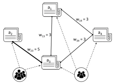
Figure 1: Modeling the relationship among news arti-cles (or events): the dash lines represent engagements of users to articles, the solid lines represent the rela-tionships between articles with weights determined by the number of common engaged users.
drawing a lot of attention from both the academic and industrial communities.
The recent literature has witnessed the success of deep learning models in detecting fake news on social media (Ma et al.,2016;Yu et al.,2017;
Ruchansky et al., 2017;Rashkin et al.,2017;Ma et al., 2018a; Kochkina et al., 2018). By lever-aging the capability of deep networks in learn-ing high-level representations, these models have achieved state-of-the-art performance on various benchmark datasets. Nevertheless, one limitation of existing deep-learning-based methods is that they often ignore the correlations among news ar-ticles, which have been proved to be effective for analysing online events (Freire et al.,2016; Fair-banks et al.,2018).
com-50 60 70 80 90 100
%
0 5 10 15 20 25 30 35 40 45 50
[image:2.595.83.278.62.207.2]edge weight
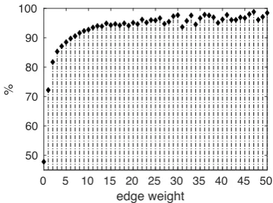
Figure 2: Percentage of edges having certain weights, which connects two articles with the same labels on the news graph constructed from the Weibo dataset (Ma et al.,2016).
mon users that engage to them, e.g., by means of tweeting, re-tweeting, commenting. An example is illustrated in Fig.1: the articlesa2 anda3 have a strong relationship as they are engaged to by5
common users, whereas, there is no relationship between the articlesa1 anda2 because there is no user engage to both of them. With this modeling, we can construct a news graph, where each node corresponds to an article and an edge encodes the relationship between two articles.
Our underlying assumption is that if there exists a strong relationship between two articles, they are likely to share the same labels. To verify this assumption, we calculate the percentages of the edges that connect two articles with the same la-bels, among those whose weights are equal to cer-tain values, and plot the results for the news graph constructed from the Weibo dataset (Ma et al.,
2016) in Fig. 2. It is clear from Fig. 2 that the higher the edge weight, the more likely it is that the corresponding articles share the same labels (fake or true). Similar patterns are observed on other datasets such as the Twitter (Ma et al.,2016) and the PHEME (Zubiaga et al., 2017) datasets. Evidently, these results support our assumption.
In order to incorporate the correlations among news articles, we formulate fake news detection as an inference problem in a Markov random field (MRF). Our motivation behind this formulation is to leverage the capability of MRF in capturing de-pendencies among random variables. We solve the resulting inference problem using the mean-field algorithm (Koller and Friedman, 2009). We then propose a method to unfold this algorithm into hidden layers that can be integrated on top
of a deep network that computes the potentials of the MRF. By doing this, we obtain our deep MRF model for detecting fake news, referred to as the DMFN model. To the best of our knowledge, this is the first integration of deep networks and MRF for detecting fake news. Our main contributions are as follows:
• We formulate fake news detection as an in-ference problem in an MRF model. This al-lows us to incorporate the correlations among news articles when deciding their credibility.
• We propose a method to unfold the mean-field algorithm into specially-designed neural network layers, and build a deep MRF model for detecting fake news.
• We carry out comprehensive experiments on widely-used datasets collected from popular social networks. Experimental results show the effectiveness of the proposed model com-pared to various state-of-the-art models.
The remainder of the paper is organized as fol-lows: we review the related work in Section2, and describe our formulation of fake news detection as an inference problem MRF in Section 3. In Sec-tion4, we describe our model in detail. We present our experimental studies in Section5 and finally draw the conclusions in Section6.
2 Related Work
Early work in fake news detection focused on find-ing a good set of features that are useful for sep-arating fake news from genuine news. Linguistic patterns, such as special characters, specific key-words and expression types, have been explored to spot fake news (Castillo et al.,2011;Liu et al.,
2015;Zhao et al., 2015). Different feature types have also been considered, such as the charac-teristics of users involved in spreading the news, e.g. the number of followers, the users’ ages and genders (Castillo et al., 2011;Yang et al.,2012), and the news’ propagation patterns (Castillo et al.,
2011;Kwon et al.,2013). Instead of relying on a single feature type, existing works normally made use of multiple types of feature at the same time.
Many works proposed to represent news articles as multivariate time series using the timestamp in-formation and to formulate fake news detection as a sequence classification problem (Ma et al.,
2016;Yu et al., 2017; Ma et al., 2018a;Liu and Brook Wu,2018;Kochkina et al., 2018). As it is common in the literature to utilize multiple types of features in detecting fake news, deep networks with multiple branches to incorporate various fea-ture types were also proposed (Ruchansky et al.,
2017;Volkova et al.,2017;Yang et al.,2018). In general, deep learning based methods yield higher accuracy compared to shallow-feature-based ap-proaches, leading to state-of-the-art performance.
The existing deep-learning models, however, often ignore the correlations among news arti-cles which haven been shown to be effective cues for analysing online news and events (Freire et al., 2016; Fairbanks et al., 2018). Freire et al. proposed a method to detect breaking news on Wikipedia by exploring the graph of related events (Freire et al.,2016). This graph is built by connecting any pair of pages on Wikipedia which were edited by the same users in a small time win-dow. In (Fairbanks et al.,2018), a graph of news was constructed by connecting the corresponding web pages using the links between them in form of html tags. The credibility of the news was assessed by applying the loopy belief propaga-tion algorithm to perform semi-supervised learn-ing on this graph. In their experiments, the authors showed that the correlations among the news, en-coded in the constructed graph, were more effec-tive than the textual content of the news for pre-dicting their credibility.
In this work, we propose a deep MRF model for fake news detection. Apart from leveraging the power of deep networks, our model incorpo-rates the correlations among news articles when determining their credibility. In this regard, our method shares a similar motivation with the graph-based methods for social event analysis as men-tioned above. Nevertheless, while these graph-based methods do not utilize any information of the news articles beyond the labels, our model is more generic and allows incorporating an arbitrary number of features.
3 Fake News Detection on MRF
We employ a Markov random field (MRF) model (Freeman et al., 2000) to incorporate the
correlations among the events due to its capabil-ity in capturing dependencies among random vari-ables. To this end, we first construct an event graphG = (V,E), withV the set of vertices and E the set of edges as described in Section 1. We then define an MRF model overG. In this model a nodekis associated with a random variableXk,
which represents the label of thek-th event. The random variables Xk,∀k ∈ {1, . . . , n} have
do-main L = {L1,L2. . .Ls}, which represent the s possible labels. For notation brevity, we re-fer to the nodes in V by their indices, namely, k∈ {1, . . . , n}. We are interested in inferring the distributionP(X)of the MRF, from which the la-bels for the events can be obtained. In the MRF, the probabilityP(X = x), with xa set of values of the random variables, is given by (Koller and Friedman,2009)
P(X = x) = 1
Z exp(−E(x)), (1) withZ the partition function ensuring a valid dis-tribution andE(x)the energy of the MRF, which has the following form
E(x) =X k∈V
Φ (xuk) +λ X
k,l∈N
Ψ (xuk,xvl). (2)
In (2),N is the set of nodes that are connected in the MRF . Theunary potential,Φ (xuk), measures the cost of assigning the label Lu to the nodek,
while thepairwise potential,Ψ(xuk,xvl), measures the cost of assigning the nodeskandlrespectively the labelsLuandLv. As such, the pairwise
poten-tials capture the dependencies among the nodes of the MRF.λis a hyperparameter.
As exactly computing P(X) is intractable, we employ the mean-field algorithm (Koller and Friedman, 2009) to approximate P(X) by a fully-factorized proposal distribution Q(X) =
Q
∀k∈VQk(Xk). Qk(Xk = Lu) is the
probabil-ity that the node k have the label Lu according to the distributionQk. DenoteQk(Xk = Lu) as
qku, the mean-field algorithm iteratively calculates qku,∀k ∈ {1, . . . , n}, u ∈ {1, . . . , s} according to (Koller and Friedman,2009)
(3) quk = 1
Zk exp
−
Φ (xuk)
+λX
l∈Nk X
v∈L
qlvΨ (xuk,xvl)
with Nk the set of nodes connected to k and
Zk = Pu∈Lqkuthe normalization factor ensuring
qku, ∀u ∈ {1, . . . , s}, add up to 1. The generic mean-field update in (3) requires the unary po-tentials and pairwise popo-tentials. In Section4, we show how we realize these potentials.
4 Deep MRF Model for Fake News Detection
In this section, we present our realizations of the unary and pairwise potentials, with which we ob-tain the final mean-field update equation. After that, we present a method to unfold the mean-field update into specially-designed neural network lay-ers, and describe our deep MRF model for fake news detection.
4.1 Computing the Unary and Pairwise Potentials
We compute the unary potentialΦ(xuk)of the MRF as the negative log likelihood:
Φ(xuk) =−lnp(Xk =Lu), (4)
with p(Xk = Lu) the likelihood that Xk has
label Lu. As such, Φ(xuk) will be high if this node is not likely to have the labelLu, and vice
versa. The likelihoodp(Xk=Lu)is computed as
p(Xk =Lu) =Fθ(Ok), whereFθ is a non-linear
function represented by a deep neural network pa-rameterized by θandOk is the observations, i.e,
features associated to thek-th event. The design of this network is described later in Section4.
The pairwise potential is computed by
Ψ(xuk,xvl) =a(k, l)×µ(u, v), (5)
where a(k, l) is the weight of the edge between the nodeskandl, namely, a(k, l)represents how strong the relationship between the nodes k and lis; andµ(u, v) is thelabel compatibility, which is calculated using the Pott model (Boykov et al.,
1998):
µ(u, v) =
(
1, ifu6=v,
0, otherwise. (6)
Substituting the pairwise potential in (5) into (3),
we obtain the final mean-field update equation:
(7) quk = 1
Zk exp
−Φ (xuk)
−λX
l∈Nk
a(k, l)X v∈L
qlv×µ(u, v)
.
We refer to the termP
v∈Lqvl ×µ(u, v)in (7) as
the compatibility transform step, and to the term P
l∈Nka(k, l) P
v∈Lqlv×µ(u, v)summing up
in-formation from the nodes connected to the nodek as themessage passingstep.
4.2 Mean-Field Updates as Neural Network Layers
We now describe a method to implement the up-date equation in (7) using operations that are com-mon in the deep learning literature. Abusing the notation, we denote also by Q ∈ Rn×s a matrix,
with an entryQk,ucorresponding to the valuequk,
i.e., the probability that the nodek has the label Lu. Denote by A ∈ Rn×n the adjacency
ma-trix, containing all the edge weights inG. We set Ak,k = 0,∀k ∈ {1, . . . , n}. We further denote
by M ∈ Rs×s a square matrix whose the entry
Mu,v corresponds the label compatibilityµ(u, v)
calculated using (6), and by Φ ∈ Rn×s the ma-trix containing the unary potentialsΦ(xuk), for all k ∈ {1, . . . , n} andu ∈ {1, . . . , s}. Φis calcu-lated by taking the logarithm ofQelement-wise.
4.2.1 The Compatibility Transform Step
The compatibility transform in (7) can be per-formed via a 1-D convolutional layer applied on the matrix Q. This convolutional layer hass fil-ters of kernel size1×s. The weights of theu-th filter are set equal to the values along theu-th row ofM. We do not employ any padding and set the stride to1. When applying this operation, theu-th filter slides vertically acrossQ, and calculates the inner product between its weights and the rows of Q. The output is denoted asQ0 ∈ Rn×s, with an entryQ0l,ugiven by
Q0l,u=X v∈L
Ql,v×Mu,v
=X v∈L
qvl ×µ(u, v), (8)
Concatenate Softmax
Conv
⨂
⨁
Softmax
Conv
⨂
⨁
Softmax Q
Φ
𝐴, 𝑀
FALSE TRUE
tf-idf
word2vec
node2vec
FC layers
FC layers
MF layers -ln
[image:5.595.100.502.59.212.2]…
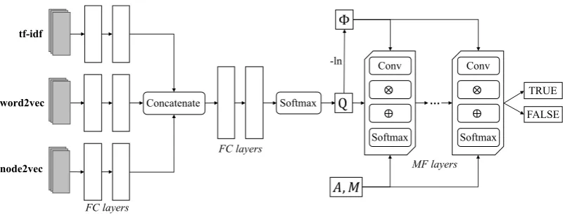
Figure 3: The architecture of the DMFN model: the first block consists of three feature branches, each with configurable numbers of fully-connected (FC) layers to process a type of feature, a concatenation layer and a number of FC layers with softmax activation function at the end to produce labels’ probability matrixQ; Each mean-field (MF) layer consists of four main operations, namely convolution (conv), matrix multiplication (⊗), point-wise addition (⊕) and the softmax function. T MF layers are stacked one after another to implement the mean-field algorithm withT iterations. All MF layers share the same set of parameters, namely, the matrix of the unary potentialsΦ, which is computed fromQ, the adjacency matrixAencoding the relationships among the input events, and the compatibility matrixM.
4.2.2 The Message Passing Step
Given the adjacency matrix A ∈ Rn×n and the
output Q0 ∈ Rn×s from the compatibility trans-form step, the message passing step can be per-formed simply by multiplying A with Q0. This multiplication results inQ00 ∈Rn×s, in which:
Q00k,u= n
X
l=1 Ak,l.Q
0
l,u
= n
X
l=1
a(k, l)X v∈L
qlv×µ(u, v). (9)
As Ak,l = 0if l 6∈ Nk, the operation in (9) is
equivalent to the message passing step in (7).
4.2.3 The Mean-field Layer
To finish the update in (7), one needs to element-wise multiply Q00 with λ, add Φ and negate the result. The exponential and normalization can be performed jointly using thesoftmax function, re-sulting in the new matrixQ∈Rn×swhose entries correspond to the values ofqukafter one mean-field iteration, for allk ∈ {1, . . . , n},u ∈ {1, . . . , s}. We can consider these operations together with those implementing the compatibility transform and the message passing steps, as the operations of specially-designed a neural network layer, which we call the mean-field (MF) layer. As all the component operations are differentiable, the op-eration implemented by the MF layer is also dif-ferentiable. Each MF layer, hence, implements
one iteration of the mean-field algorithm. Clearly, by stackingT MF layers, we can implement the mean-field algorithm withT iterations.
4.3 The DMFN Model
4.3.1 Model Architecture
The architecture of the DMFN model is illustrated in Figure3, with two blocks: the first block cor-responds to the deep network Fθ that produces the unary potentials, and the second block is com-posed ofT MF layers, which implements theT -iteration mean-field algorithm. The deep network Fθ takes as inputs several feature types extracted
to represent the given set of events. Each fea-ture type is processed by a feafea-ture branch with a number of fully-connected (FC) layers. The outputs of the last layers in all feature branches are concatenated to produce high-level represen-tations for all the events. These represenrepresen-tations are then fed to another set of FC layers and a softmax function to produce the label probabili-ties. These label probabilities form the matrixQ, as described in Section 4.2. All the FC layers in the model are followed by a batch normalization layer (Ioffe and Szegedy, 2015), a ReLU activa-tion funcactiva-tion (Glorot et al.,2011), and the dropout regularization (Srivastava et al.,2014).
among the given events, and the label compatibil-ity matrix M. The first MF layer takes as input the matrix Q, whereas, the later MF layers oper-ate on the outputs from their previous MF layers. The output after the last MF layer is the final la-bel probabilities predicted for the given events. It should be noted that the parameters of the MF lay-ers are pre-computed and shared. As such, adding MF layers after the layers in the first block does not increase the the risk of overfitting of the model.
4.3.2 Feature Extraction
We extract multiple types of features to capture the characteristics of the events, namely, the tex-tual contents and social engagements. For the textual features, we first group all the tweets re-lated to an event into a document. We pre-process the documents by removing stop words, converting the words into lower case and tokeniz-ing them. From the pre-processed documents, we extract the term frequency - inverse docu-ment frequency (tf-idf) (Wu et al., 2008), and
word2vec (Mikolov et al., 2013) feature vectors. We use the word2vec model pre-trained on the Google News dataset to map each word in a doc-ument to a 300−dimensional embedding vector, and then obtain the embedding for the document by taking the average of the word embeddings.
We use a graph embedding technique to capture the social engagements associated to the events. Concretely, we first build a graph of users from the given dataset. Two users are connected by an edge if they engage to at least one event in common, with the edge’s weight determined by the total number of common engaged events. We then employ thenode2vecalgorithm (Grover and Leskovec, 2016) to learn an embedding for each user. The social engagement feature of an event is then calculated by taking the average of the em-beddings of all users engaged to it. It is worth noting that the graph of users used in this step is different from the graph of events, constructed as described in Section1.
4.3.3 Training and Testing the DMFN Model
We employ the weighted cross entropy loss func-tion to train the DMFN model. When calcu-lating the loss, the weight given to the training samples of a particular label is inversely propor-tional to the number of samples in the current batch which have this label. This technique is highly beneficial when dealing with imbalanced
dataset, e.g., the PHEME dataset (Zubiaga et al.,
2016). The model’s parameters are learned by us-ing the SGD algorithm with the Adam parameter update (Kingma and Ba,2015).
At the testing stage, we select for the testing eventk the label Luˆ ∈ Lwith uˆ determined by
ˆ
u = arg maxu∈{1,...,s}qku. As we want to utilize
the correlations among events in the prediction, we provide an adjacency matrix encoding the relation-ships among a set of events and run a forward pass with all their features as input. Without the adja-cency matrix or when setting the adjaadja-cency matrix to the identity matrix, the model predicts the labels for each events without considering their correla-tions.
5 Experiments
5.1 Experimental Settings
We employ three well-known benchmark datasets, namely the Twitter, Weibo (Ma et al., 2016) and PHEME datasets (Zubiaga et al., 2017) for our experiments. The Twitter dataset consists of 992
events, involving233.7thousand users and592.4
thousand tweets. The Weibo dataset is larger, with4,664events,2.8million users and3.8 mil-lion posts. Events in these datasets are labeled as eitherfake ortrue, and the two labels are rel-atively balanced. The PHEME dataset consists of5,802comment threads collected from Twitter, with approximately103thousand tweets in total. This dataset is imbalanced, with1,972threads la-beled asrumourand3,830threads labeled as non-rumour.
5.2 Hyperparameter Selection
For the DMFN model, we employ one hidden layer in each feature branch, and one hidden layer after the concatenation layer, all with 100 hid-den units. We train the model for maximum100
epochs with learning rate0.001and stop training early if the validation loss does not improve over the average of those of the previous25epochs. To control overfitting, we employ dropout with high dropping rate of0.9.
experi-λ 0.005 0.050 0.100 0.500
[image:7.595.87.274.139.165.2]Weibo 0.958 0.960 0.959 0.949
Table 1: Accuracy of the DMFN model when varying
λon the Weibo datasets (Ma et al.,2016).
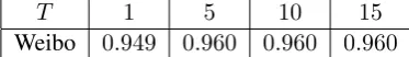
T 1 5 10 15
Weibo 0.949 0.960 0.960 0.960
Table 2: Accuracy of the DMFN model when varying
T on the Weibo datasets (Ma et al.,2016).
ment with different values ofλ. The result of this is presented in Table1.
Fixing λ to 0.05, we experiment with differ-ent number of MF layers by varyingT. The re-sults are summarized in Table2. As can be seen from the table, employing multiple MF layers im-proves the results over just one MF layer. Even though we still observe improvements in the per-formance with more than5MF layers, the differ-ence is small. As a result, we selectT = 5as it produces the best trade-off between accuracy and computational complexity.
5.3 Experimental Results
We compare the results of different models in two experimental settings, namely late detection and
early detection. The former setting allows the models to use all the available users posts in the entire time span of the given datasets, whereas in the latter setting, the models are only allowed to use posts that have appeared within a specific deadline (in hours) since the appearances of the events.
5.3.1 Late Detection Setting
We compare the results of the proposed models in the late detection setting with those of refer-ence models, including the decision tree classifier (DTC) (Castillo et al.,2011), the SVM classifier (SVM-RBF) (Yang et al.,2012), the random for-est classifier (RFC) (Kwon et al.,2013), the SVM classifier with timeseries features (SVM-TS) (Ma et al.,2015), the 2-layer GRU model (GRU-2) (Ma et al.,2016) and the convolutional neural network (CAMI) (Yu et al.,2017), the Tree-structured Re-cursive Neural Networks (TD-RvNN) (Ma et al.,
2018b), and the CRF and Naive Bayes classifiers in (Zubiaga et al., 2017). The performance of the models is assessed using four metrics, namely, accuracy, average precision, average recall and
macro F1 score. Similar to (Yu et al.,2017), on the Twitter and Weibo datasets, we randomly reserve
10%of the samples for parameter tuning and per-form four-fold cross validation on the remaining. On the PHEME dataset, we follow the leave-one-event-out approach as in (Zubiaga et al., 2017). We report the average results for the models.
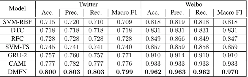
The results for different models on the Twit-ter and the Weibo datasets (Ma et al., 2016) are shown in Table 3. On these two datasets, we do not include the results of the TD-RvNN model (Ma et al., 2018b) as this model requires a tree-like connections among the tweets to repre-sent an event. As can be seen from the table, the DMFN model consistently outperforms the refer-ence models on both datasets. The results of all the models are better on the Weibo dataset than on the Twitter dataset. This is possibly because num-ber of posts available on the Weibo dataset is much larger than that available on the Twitter dataset.
The results on the PHEME dataset is illustrated in Table.4. As this dataset is imbalanced, the pre-diction accuracy is not a good metric for compar-ison. Similar to (Zubiaga et al., 2017), we fo-cus on the other metrics, namely, precision, re-call and macro F1 score in the comparison. The CRF model with content features (Zubiaga et al.,
2017) yields the highest precision, whereas the Naive Bayes classifiers yield the highest recalls.. While the reference models are either biased to-ward high precision or high recall scores, the DMFN model produces more balanced precision and recall, and the best Macro F1 score. The DF-RvNN model (Ma et al.,2018a) also achieves bal-anced precision and recall, nevertheless its perfor-mance is lower than that of the DMFN model in all metrics (with p-values of0.004,0.04,0.03 respec-tively for the precision, recall and macro f1 scores in a pairwise t-test).
On the PHEME dataset, the average number of tweets per event is 17.8, which is much smaller than those on the Twitter and Weibo datasets (805
Model Twitter Weibo
Acc. Prec. Rec. Macro F1 Acc. Prec. Rec. Macro F1
SVM-RBF 0.715 0.720 0.710 0.709 0.818 0.819 0.818 0.818
DTC 0.718 0.718 0.718 0.718 0.831 0.831 0.831 0.831
RFC 0.728 0.728 0.728 0.728 0.849 0.866 0.849 0.847
SVM-TS 0.745 0.741 0.741 0.740 0.857 0.859 0.858 0.859
GRU-2 0.757 0.760 0.757 0.771 0.910 0.914 0.910 0.910
CAMI 0.777 0.782 0.777 0.776 0.933 0.933 0.933 0.933
DMFN 0.800 0.803 0.803 0.799 0.962 0.963 0.962 0.970
Table 3: Results for different models on the Twitter and Weibo datasets (Ma et al.,2016).
Model Prec. Rec. Macro F1
Naive Bayes Content 0.309 0.723 0.433
CRF Content 0.683 0.545 0.606
Naive Bayes Content + Social 0.310 0.723 0.434
CRF Content + Social 0.667 0.556 0.607
TD-RvNN 0.616 0.612 0.609
DMFN 0.667 0.670 0.657
Table 4: Results for different models on the PHEME datasets (Zubiaga et al.,2017).
Model Twitter Weibo PHEME
Acc. Macro F1 Acc. Macro F1 Acc. Macro F1
DMFN-base 0.763 0.762 0.944 0.944 0.682 0.607
DMFN-separate 0.789 0.788 0.958 0.959 0.690 0.641
[image:8.595.95.506.62.191.2]DMFN 0.800 0.799 0.962 0.970 0.703 0.657
Table 5: Results of different variants of the DMFN model on the three datasets.
1e−4,2e−4and6e−5respectively on the Twitter, Weibo and PHEME datasets.
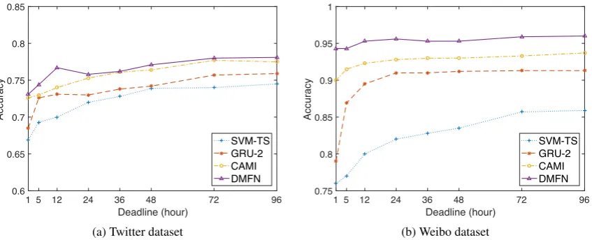
5.3.2 Early Detection Setting
We perform the early detection experiments on the Twitter and Weibo datasets with different deadlines, in{1,5,12,24,36,48,72,96}(hours). Fig. 4a and Fig. 4b illustrate the results on the Twitter and the Weibo datasets, respectively. As can be seen, on both datasets, the DMFN model performs the best among the selected models, followed by the CAMI model. On the Weibo dataset, the average number of posts per event is approximately 168, 353, 497 within the 1-hour, 5-hour and 12-hour deadlines respectively.These figures suggest that Weibo users are responsive and quickly react to a newly broadcasted event. The large number of posts per event, even at 1-hour deadline, gives enough information for the DMFN, as well as the CAMI models to produce good results, even within short deadlines.
5.3.3 The Effects of Jointly Training the Deep Network with Mean-field Inference
1 5 12 24 36 48 72 96
Deadline (hour)
0.6 0.65 0.7 0.75 0.8 0.85
Accuracy
SVM-TS GRU-2 CAMI DMFN
(a) Twitter dataset
1 5 12 24 36 48 72 96
Deadline (hour)
0.75 0.8 0.85 0.9 0.95 1
Accuracy
SVM-TS GRU-2 CAMI DMFN
[image:9.595.90.514.62.234.2](b) Weibo dataset
Figure 4: Accuracy of different models when considering only posts within specific deadlines on the Twitter and Weibo datasets.
the benefits of unfolding the MF inference and in-corporate it on top of the base network.
6 Conclusion
We formulated the fake news detection on social media as an inference problem in an MRF model that can be solved using the mean-field algorithm. By translating each update step in this algorithm into common operations in the deep learning lit-erature, we can unfold it into hidden layers that can be integrated on top of another deep neural network. This results in our deep MRF model (DMFN) for detecting fake news. As such, the DMFN carries the advantages of both deep neural networks in learning high-level representations, and of MRF in incorporating correlations among the news articles. Experiments on well-known benchmark datasets show that the proposed model consistently improves over the state of the art in fake news detection in both the late and early de-tection settings.
Acknowledgments
The authors acknowledge the financial support from the Vrije Universiteit Brussel (PhD bursary -Duc Minh Nguyen), the Fonds Wetenschappelijk Onderzoek Vlaanderen (FWO) and the Franc-qui Foundation (2016-2017 International FrancFranc-qui Chair - Robert Calderbank).
References
Yuri Boykov, Olga Veksler, and Ramin Zabih. 1998. Markov random fields with efficient
approxima-tions. InIEEE Conference on Computer Vision and Pattern Recognition (CVPR), pages 648–655.
Carlos Castillo, Marcelo Mendoza, and Barbara Poblete. 2011. Information credibility on twitter. In ACM International Conference on World Wide Web (WWW), pages 675–684.
James Fairbanks, Natalie Fitch, Nathan Knauf, and Er-ica Briscoe. 2018. Credibility assessment in the news : Do we need to read ? InMisinformation and Misbehavior Mining on the Web Workshop (MIS2), pages 1–8.
William T. Freeman, Egon C. Pasztor, and Owen T. Carmichael. 2000. Learning low-level vision. Inter-national Journal of Computer Vision, 40(1):25–47.
Ana Freire, Matteo Manca, Diego Saez-Trumper, David Laniado, Ilaria Bordino, Francesco Gullo, and Andreas Kaltenbrunner. 2016. Graph-based break-ing news detection on wikipedia. In AAAI Con-ference on Web and Social Media (ICWSM) Work-shops, pages 1–2.
Xavier Glorot, Antoine Bordes, and Yoshua Bengio. 2011. Deep sparse rectifier neural networks. In In-ternational Conference on Artificial Intelligence and Statistics (AISTATS), pages 315–323.
Aditya Grover and Jure Leskovec. 2016. Node2vec: Scalable feature learning for networks. In ACM SIGKDD International Conference on Knowledge Discovery and Data Mining, pages 855–864.
Sergey Ioffe and Christian Szegedy. 2015. Batch nor-malization: Accelerating deep network training by reducing internal covariate shift. In International Conference on Machine Learning (ICML), pages 448–456.
Elena Kochkina, Maria Liakata, and Arkaitz Zubiaga. 2018. All-in-one: Multi-task learning for rumour verification. In International Conference on Com-putational Linguistics (COLING).
Daphne Koller and Nir Friedman. 2009. In Probabilis-tic Graphical Models: Principles and Techniques. MIT Press.
Philipp Kr¨ahenb¨uhl and Vladlen Koltun. 2011. Effi-cient inference in fully connected crfs with gaussian edge potentials. InAdvances in Neural Information Processing Systems (NIPS), pages 109–117.
Sejeong Kwon, Meeyoung Cha, Kyomin Jung, Wei Chen, and Yajun Wang. 2013. Prominent features of rumor propagation in online social media. InIEEE International Conference on Data Mining (ICDM), pages 1103–1108.
Xiaomo Liu, Armineh Nourbakhsh, Quanzhi Li, Rui Fang, and Sameena Shah. 2015. Real-time rumor debunking on twitter. In ACM International on Conference on Information and Knowledge Man-agement (CIKM), pages 1867–1870.
Yang Liu and Yi-Fang Brook Wu. 2018. Early detec-tion of fake news on social media through propaga-tion path classificapropaga-tion with recurrent and convolu-tional networks. In AAAI Conference on Artificial Intelligence, pages 1–8.
Jing Ma, Wei Gao, Prasenjit Mitra, Sejeong Kwon, Bernard J. Jansen, Kam-Fai Wong, and Meeyoung Cha. 2016. Detecting rumors from microblogs with recurrent neural networks. InJoint Conference on Artificial Intelligence (IJCAI), pages 3818–3824.
Jing Ma, Wei Gao, Zhongyu Wei, Yueming Lu, and Kam-Fai Wong. 2015. Detect rumors using time se-ries of social context information on microblogging websites. In ACM International on Conference on Information and Knowledge Management (CIKM), pages 1751–1754.
Jing Ma, Wei Gao, and Kam-Fai Wong. 2018a. Detect rumor and stance jointly by neural multi-task learn-ing. In The Web Conference (WWW), pages 585– 593.
Jing Ma, Wei Gao, and Kam-Fai Wong. 2018b. Rumor detection on twitter with tree-structured recursive neural networks. In Annual Meeting of the Asso-ciation for Computational Linguistics (ACL), pages 1980–1989.
Tomas Mikolov, Ilya Sutskever, Kai Chen, Greg Cor-rado, and Jeffrey Dean. 2013. Distributed repre-sentations of words and phrases and their composi-tionality. InInternational Conference on Neural In-formation Processing Systems (NIPS), pages 3111– 3119.
Hannah Rashkin, Eunsol Choi, Jin Yea Jang, Svit-lana Volkova, and Yejin Choi. 2017. Truth of varying shades: Analyzing language in fake news
and political fact-checking. InConference on Em-pirical Methods in Natural Language Processing (EMNLP), pages 2931–2937.
Natali Ruchansky, Sungyong Seo, and Yan Lin. 2017. CSI : A hybrid deep model for fake news detection. InACM International on Conference on Information and Knowledge Management (CIKM), pages 797– 806.
Kai Shu, Amy Sliva, Suhang Wang, Jiliang Tang, and Huan Liu. 2017. Fake news detection on social me-dia: A data mining perspective. SIGKDD Explo-rations Newsletter, 19(1):22–36.
N. Srivastava, G. E. Hinton, A. Krizhevsky, I. Sutskever, and R. Salakhutdinov. 2014. Dropout: a simple way to prevent neural networks from overfitting. Journal of machine learning research, 15:1929–1958.
Svitlana Volkova, Kyle Shaffer, Jin Yea Jang, and Nathan Hodas. 2017. Separating facts from fiction: Linguistic models to classify suspicious and trusted news posts on twitter. In Annual Meeting of the Association for Computational Linguistics (ACL), pages 647–653.
Ho Chung Wu, Robert Wing Pong Luk, Kam Fai Wong, and Kui Lam Kwok. 2008. Interpreting TF-IDF term weights as making relevance deci-sions. ACM Transactions on Information Systems, 26(3):13:1–13:37.
Fan Yang, Yang Liu, Xiaohui Yu, and Min Yang. 2012. Automatic detection of rumor on sina weibo. In ACM SIGKDD Workshop on Mining Data Seman-tics, pages 13:1–13:7.
Yang Yang, Lei Zheng, Jiawei Zhang, Qingcai Cui, Xi-aoming Zhang, Zhoujun Li, and Philip S. Yu. 2018. TI-CNN : Convolutional neural networks for fake news detection.ArXiv e-prints 1806.00749.
Feng Yu, Qiang Liu, Shu Wu, Liang Wang, and Tieniu Tan. 2017. A convolutional approach for misinfor-mation identification. InInternational Joint Confer-ence on Artificial IntelligConfer-ence (IJCAI), pages 3901– 3907.
Zhe Zhao, Paul Resnick, and Qiaozhu Mei. 2015. En-quiring minds: Early detection of rumors in so-cial media from enquiry posts. In ACM Inter-national Conference on World Wide Web (WWW), pages 1395–1405.
Arkaitz Zubiaga, Maria Liakata, and Rob Procter. 2017. Exploiting context for rumour detection in so-cial media. InSocial Informatics, pages 109–123.