Supply Chain Management in a Dairy
Industry – A Case Study
K. Venkata Subbaiah , Member, IAENG, K. Narayana Rao K. Nookesh babu
ABSTRACT -Supply chain management is the plan and
control of material and information flow among suppliers, facilities, warehouses and customers with the objectives of minimization of cost, maximization of customer services and flexibility. The supply chain of a business process comprises mainly five activities viz., Purchase of materials from suppliers, transportation of materials from suppliers to facilities, production of goods at facilities, transportation of goods from facilitates to ware houses and transportation of goods from ware houses to customers.
In this paper, a supply chain model is developed for a dairy industry, located in Andhra Pradesh, India. The supply chain includes four echelons namely raw milk suppliers, plant, warehouse and customers. In this model, emphasis is mainly on production and distribution activities, with a view to find out purchase plan of raw milk, production plan of product mix and transportation plan of the products.
Index Terms- Supply chain management,
Transportation, Production plan, Customer zones.
I. INTRODUCTION
Supply chain management (SCM) is a rapidly evolving area of interest to academicians and business management practitioners alike. Coordinating the external and internal activities of a firm is the basic philosophy of supply chain management. It is about managing the entire process in a collective and unified fashion.
Most of the manufacturing firms are organized as networks of manufacturing and distribution facilities that procure raw materials transform them into intermediate and finished
K. Venkata Subbaiah is with Department of Mechanical Engineering, Andhra University, Visakhapatnam, India. Phone: +91-891-2536486 (R), +91-09848063452 (M) e-mail: [email protected]
K. Narayana Rao is with Department of Mechanical Engineering, Government Polytechnic, Visakhapatnam. K.Nookesh babu is with Department of Mechanical Engineering, Andhra University, Visakhapatnam.
products and distribute the finished products to customers. The simplest network consists of facilities which perform procurement, manufacturing and distribution. These networks are called value added chains or supply chains.
A supply chain consists of all stages involved directly or indirectly in fulfilling a customer request. The supply chain not only includes the manufactures and suppliers but also retailers and customers themselves with in each organization.
deterministic model for supply chain management with an objective function containing the cost and time elements. Even though supply chain management is relatively new, the idea of co-ordinate planning is not new. The study of multi-echelon inventory/distribution systems began as early as 1960 by Clark and Scarf [2]. Since then many researchers have investigated multi echelon inventory and distribution systems. Less research has been aimed at co-ordination of procurements, production and distribution systems. In this paper an attempt has been made to develop a coordinated supply chain-planning model with procurement, production and distribution systems.
II. MODEL FORMULATION
The proposal of the model is to find an optimal strategic plan for an integrated supply chain model.
Notations
MCtvp Cost of material p purchased by vendor v at time t
PCtfg
Production
cost of goods g produced by facility f at time tVFTCtvp Transportation cost of material p Transported from vendor v to facility f at time t
FWTCtfwg Transportation cost of goods g transported from facility f to ware house w at time t
WZTCtwcg Transportation cost of goods g transported from ware house w to customer location c at time t FMICtfp Inventory cost of mterial p
of facility f at time t FGICtfg Inventory cost of goods g
of facility f at time t
WICtwg Inventory cost of goods g of warehouse w at time t
BOMgp Amount of material p needed for producing goods g
AVtvp The amount of material p purchased by vendor v at time t Rtvfp The amount of material p which
vendor v Transported of facility f at time t.
AFtfp The inventory of material p in the facility f at time t
Rtfg Amount of good g which facility f produced at time t
AFtfg The inventory of goods g at facility f at time t.
Rtfwg The amount of goods g which facility f transported to ware house w at time t.
AWtwg The inventory of good g in the ware house w at time t.
Rtwcg The amount of good g which ware house w transported to
customer c at time t. ACtcg The demand of goods g by
customer c at time t.
Assumptions
1. Capacities of vendors are fixed. 2. Demand is deterministic.
3. Variable cost per unit production is constant
Mathematical model
This model consists of four echelons namely Suppliers, Plants, Distribution Centers (DCs), and Customer zones (CZs).
A multi-objective function is formulated to minimize cost subject to supplies, plant and distribution capacities, production and distribution through put limits and customs demand requirements. Total cost includes fixed costs of production and distribution, variable costs of production, distribution and transportation.
Various costs involved in the supply chain are
1. Material Cost = tvp AVtvp vp
MC *
∑
2. Production cost = tfg Rtfg fg
PC *
∑
3. Transportation cost =
* * *
VFTCtvfp Rtvfp FWTCtfwg Rtfwg WCTCtwcg Rtwcg
vfp fwg wcg
∑ + ∑ + ∑
4. Inventory cost =
* * *
tfp tfg twg
FMIC AFtfp FGIC AFtfg WIC AWtwg
ft fg wg
∑ + ∑ + ∑
The objective function of the model is to minimize the total cost associated with the supply chain which includes material, production, transportation and inventory costs.
Minimize Z=
* * *
* * *
* *
tfp
tfg twg
MCtvp AVtvp PCtfg Rtfg VFTCtvfp Rtvfp
vsp fg vfp
FWTCtfwg Rtfwg WCTCtwcg Rtwcg FMIC AFtfp
fwg wcg ft
FGIC AFtfg WIC AWtwg
fg wg
∑ + ∑ + ∑
∑ ∑ ∑
+ + +
∑ ∑
The above stated problem is solved subjected to the following constraint set.
1. Upper – Lower bound restrictions
0 ≤ Rtvfp ≤ Rtvfp _ UPbound 0 ≤ Rtfwg ≤ Rtfwg _ UPbound 0 ≤ Rtwcg ≤ Rtwcg _ UPbound
Rtfg _ LPbound ≤ Rtfg ≤ Rtfg _ UPbound etvf =1; ettw =1; etvc=1;
2. Flow Conservative restrictions
, ,
tvfp tvp
t
R
=
LV
∀
t v p
∑
( vf)
*
tfp t et vfp gp tfg
v g
AF
+
∑
R
−−
∑
BOM
R
( 1)t fp
, ,
AF
+t f p
=
∀
( ) ( 1)
, ,
fw fwg twcg
twg t et t wg
f c
AW
R
R
AW
t w g
− +
+
−
=
∀
∑
∑
(t etwc)wcg tcg
, ,
wR
−=
AC
∀
t c g
∑
III. CASE STUDY
The above developed model is applied to Visakha Dairy situated in Andhra Pradesh, India. The above dairy has six vendors located at Vsiahapatnam, Vizianagaram, Tuni, Ramabadrapuram, Narsipatnam and Srikakulam. It has two facilities located at Visakhapatnam and kakinada to meet the customer demands. Five warehouses are situated at Visakapatnam, Vizianagaram, Srikakulam Kakinada and Rajahmundry. Its customer locations are situated at Visakhapatnam, Vizianagaram, Srikakulam, Kakinada and Rajamundry.
The input data required for the design of supply chain for the above stated industry is given below.
Input Data
Material Cost
v p
1 2 3 4 5 6
1 1140 1160 991 1135 872 1056
Vendor to facility transportation cost
v f
1 2 3 4 5 6
1 3.26 26.33 36.24 28.56 84.8 33.35 2 32.98 6.02 66.24 55.56 103.8 3.26
Facility to ware house transportation cost
For facility1 g
w
1 2 3 4 5 6
1 3.26 3.26 3.26 3.26 3.26 3.26 2 11.9 11.9 11.9 11.9 11.9 11.9 3 13.6 13.6 13.6 13.6 13.6 13.6 4 8.9 8.9 8.9 8.9 8.9 8.9 5 7.56 7.56 7.56 7.56 7.56 7.56
For facility 2 g
w
1 2 3 4 5 6
1 10.9 10.9 10.9 10.9 10.9 10.9 2 4.52 4.52 4.52 4.52 4.52 4.52 3 3.26 3.26 3.26 3.26 3.26 3.26 4 19.8 19.8 19.8 19.8 19.8 19.8 5 18.4 18.4 18.4 18.4 18.4 18.4
Ware House to customer transportation cost
c w
1 2 3 4 5
1 0 11.9 13.16 8.9 7.56
2 13.26 0 1.26 3 4.1 3 9.96 1.3 0 4.26 5.56 4 6.74 3 4.26 0 1.24 5 4.3 4.34 5.36 1.24 0
In the above table the transportation cost for good 1 is shown and the same table repeats for the remaining goods.
Inventory carrying cost at the facility for the raw material and goods are considered as Zeros.
Inventory const at warehouse
g
w 1 2 3 4 5 6
Capacities of Vendors (in thousands)
v p
1 2 3 4 5 6
1 178 43 325 45 22 20
Capacities of facilities for producing different goods
g
f 1 2 3 4 5 6
1 25000 11000 7500 4000 4000 32000 2 4000 15000 0 150 4000 30000
Capacities of ware house to hold different products
g w
1 2 3 4 5 6
1 25000 100000 7000 3000 4000 25000 2 1500 5000 0 0 1000 20000 3 1500 4000 0 500 2000 8000
4 1000 3000 0 0 1000 6000
5 0 500 500 500 300 5000
Demands for different goods at different customer locations
g
c 1 2 3 4 5 6
1 23760 10903 7000 3199 3624 23726
2 1072 4624 0 0 304 16684
3 1254 3564 0 106 2076 7352 4 962 3234 0 0 806 6210 5 0 195 0 158 193 4659
The Problem is solved using LINGO student version package.
IV. RESULTS AND DISCUSSIONS
The optimal solution for the model is
Table I: Quantities of material to be procured version different vendors.
v
p 1 2 3 4 5 6
[image:4.595.302.526.263.313.2]1 106565 43000 32500 0 22000 29000
Table II: Quantities of goods transported from vendors to facilities
v
f 1 2 3 4 5 6
1 106565 9850 32500 0 22000 0 2 0 33150 0 0 0 29000
Table III: Amounts of goods produced at both the facilities
g f
1 2 3 4 5 6
[image:4.595.301.529.360.571.2]1 23048 105920 7000 3313 2003 28631 2 4000 1500 0 150 4000 3000
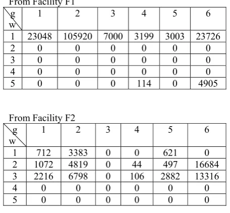
Table IV: Amounts of goods transported from facilities to warehouse
From Facility F1 g
w
1 2 3 4 5 6
1 23048 105920 7000 3199 3003 23726 2 0 0 0 0 0 0 3 0 0 0 0 0 0 4 0 0 0 0 0 0
5 0 0 0 114 0 4905
From Facility F2 g
w
1 2 3 4 5 6
[image:4.595.64.290.427.512.2]1 712 3383 0 0 621 0 2 1072 4819 0 44 497 16684 3 2216 6798 0 106 2882 13316 4 0 0 0 0 0 0 5 0 0 0 0 0 0
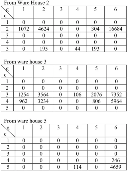
Table V: Amounts of goods to be transported from ware houses to customer Zones.
From ware house 1 g
c
1 2 3 4 5 6
1 23760 109303 7000 3199 3624 23726
2 0 0 0 0 0 0
3 0 0 0 0 0 0
4 0 0 0 0 0 0
[image:4.595.302.527.625.714.2]From Ware House 2 g
c 1 2 3 4 5 6
1 0 0 0 0 0 0 2 1072 4624 0 0 304 16684 3 0 0 0 0 0 0 4 0 0 0 0 0 0 5 0 195 0 44 193 0
From ware house 3 g
c 1 2 3 4 5 6
1 0 0 0 0 0 0 2 0 0 0 0 0 0 3 1254 3564 0 106 2076 7352 4 962 3234 0 0 806 5964 5 0 0 0 0 0 0
From ware house 5 g
c 1 2 3 4 5 6
1 0 0 0 0 0 0
2 0 0 0 0 0 0
3 0 0 0 0 0 0
4 0 0 0 0 0 246
[image:5.595.63.288.107.408.2]5 0 0 0 114 0 4659
Table I represents the procurement plan which indicates quantities of raw materials to be procured from different vendors. As both the material cost and transportation costs to both the facilities is high from vendor 4 (i.e., Ramabadrapuram) and the demand for the raw material can be fulfilled by the remaining vendors, raw material should not be procured from the vendor 4. Table III represents the production plan for the optimal product mix. It gives us the quantities of material to be produced by both the facilities considering the demands of the customers and their transportation cost.
Table II, IV and V represent the transportation plans for the plant. Table II shows the quantities of material to be transported from different vendors to both the facilities. Table IV shows the quantities of different goods to the shipped to the warehouses from both the facilities. Table V shows the quantities of different goods to be transported from different warehouse to all the customer locations. The Transportation cost to ware house 4 is very high from both the facilities and it is also very far away from all the customer zones, so the warehouse 4 is discarded from the plan. From the above obtained plans the total cost of the supply chain is calculated as Rs.27, 41,039/- per one time period (i.e.12 hours). The obtained value is
Rs.2,02,539/- less than the existing cost.
V. CONCLUSIONS
In this paper supply chain network is designed for a dairy industry. This network includes material purchase plan, production plan, inventory plan and transportation plan. From the results it is observed that the total cost of the supply chain is 9.8 percent lesser than the existing cost. This model can be extended to varying demand and costs. This can also be applied to fast moving consumer goods.
REFERENCES
[1.] Supply-Chain Council, Inc., 1998, Overview of the SCOR Model V2.0, www.supply-chain.org.
[2.] Clark, A. J., and Scarf, H., 1960, Optimal Policies for a MultiiEchelon Inventory Problem, Management Science, Vol. 6,475-490.
[3.] Cohen, M. A., and Huchzermeier, A., 1998, Global Supply Chain Management: A survey of Research and Applications, Quantitative Models for Supply Chain Management, Kulwer academic publishers .
[4.] Ehap H. Sabri and Benita M. Beamon 2000, A Multi-Objective Approach to Simultaneous Strategic and Operational Planning in Supply Chain Design, Omega Vol. 28, NO.5, 581-598.
[5.] Ganeshan, R , Stephens, P., Jack, E . , and Magazine, M., 1999, A taxonomic review of supply chain management research, Quantitative models for supply chain management. The Netherlands: Kluwer academic publishers, 839 - 879.
[6.] Pyke , D.F . , and Cohen, M . A . , 1994, Multi product integrated production distribution system , European journal of operations research. Vol 74 , No I , 18 - 49. [7.] T. H. Lee and S.H . Kim. , 2000,optimal
production distribution planning in supply chain management using a hybrid simulation Analytic approach.
[8.] Thomas D. 1. and P. M. Griffin. , 1996, Co coordinated supply chain management. European journal of operation research, 94: 1- 15.