doi:10.4236/wsn.2011.38030 Published Online August 2011 (http://www.SciRP.org/journal/wsn)
Sensor Scheduling Algorithm Target Tracking-Oriented
Dong Mei Yan, Jin Kuan Wang
School of Information Science and EngineeringNortheastern University, ShenYang, Liaoning Province, China E-mail: dmy_125@163.com
Received June 17, 2011; revised July 21, 2011; accepted July 31, 2011
Abstract
Target tracking is a challenging problem for wireless sensor networks because sensor nodes carry limited
power recourses. Thus, scheduling of sensor nodes must focus on power conservation. It is possible to extend
the lifetime of a network by dynamic clustering and duty cycling. Sensor Scheduling Algorithm Target
Tracking-oriented is proposed in this paper. When the target occurs in the sensing filed, cluster and duty
cycling algorithm is executed to schedule sensor node to perform tracking task. With the target moving, only
one cluster is active, the others are in sleep state, which is efficient for conserving sensor nodes’ limited
power. Using dynamic cluster and duty cycling technology can allocate efficiently sensor nodes’ limited
energy and perform tasks coordinately.
Keywords
:
Wireless Sensor Network, Sensor Scheduling, Target Tracking, Collaborative Signal Processing,
Dynamic Clustering
1. Introduction
Wireless sensors network is becoming an important topic of research with development of digital circuitry, wire-less communications and Micro Electro Mechanical Sys- tems, which is composed of many tiny sensor nodes built in one or more sensors, computation and communication unit, and a power supply. Sensor nodes may be deployed to perform measurements in environments including in-strumentation of rotating machinery and so on or moni-toring the movements of small animal [1].
Wireless sensor network is a power-limited and multi- user distributed system, so it is necessary to make sensor nodes operate collaboratively. CSP (collaborative signal processing) is a new research field in wireless sensor networks aiming at developing new algorithms for processing massive information sensed by sensor nodes. It is critical for wireless sensor network using CSP to dynamically allocate resources among sensor nodes [2].
A typical application in wireless sensor networks is target tracking, such as security surveillance and wildlife habitat monitoring. Target tracking contains a lot of col-laboration between individual sensors to perform com-plex signal processing algorithms such as Kalman filter-ing, Bayesian data fusion and other optimal algorithm. Thus, energy management is a key task during target moving, which affects energy consumption and network lifetime. Cooperative strategies for target tracking are
based on the following idea: with target moving, a set of nodes are selected to perform task, and the other nodes can be turned off for saving energy. The node selection is based on special algorithm considering nodes’ residual energy, distance form target and so on. Thus, considera-ble energy can be potentially conserved [3,4].
Xu Y et al. proposed a geographical adaptive fidelity (GAF) algorithm that keeps energy by identifying nodes equivalent from a routing perspective. GAF can keep a constant level of fidelity by turning off unnecessary nodes. Simulation shows that network lifetime increases proportionally to node density. GAF can be used for ex-tending network lifetime by exploiting redundancy in order to keep energy [5].
Jianyong Lin et al. presented an adaptive multisensor scheduling scheme for target tracking in Wireless Sensor Network, which is divided into three steps. First, the sampling interval is set by a predetermined tracking ac-curacy value. Then, some sensors are chosen to form a cluster for performing task. Last, the cluster head is de-termined based on the predicted energy consumption. A Monte Carlo method is employed to predict approx-imately the target state. The proposed scheme can not only reduce the energy consumption and improves the tracking reliability, but also resist the uncertainty of the process noise form simulation results [6].
opts honeycomb structure to increase one-hop coverage area. When the target occurs in the sensing filed, cluster and duty cycling algorithm is executed to schedule sensor node to perform tracking task. The Kalman filter is em-ployed to estimate next possible location of target. With the target moving, only one cluster is active, the other are in sleep state, which is efficient for conserving sensor nodes’ limited power. Using dynamic cluster and duty cycling technology can make good use of each sensor nodes’ li-mited energy and perform tasks coordinately.
2. Prolonging the Lifetime of Sensor
Network
2.1. Energy Consumption of Sensor Nodes
A sensor node consists of a sensing unit, a processing unit, a transceiver unit and a power unit as shown in
Figure 1, which a limited energy (< 0.5 Ah, 1.2 V). Moreover, sometimes it may be impossible to replace power resources. So, sensor node lifetime is mainly de-cided by battery lifetime. Power conservation and power management of sensor nodes is a key problem for wire-less sensor network.
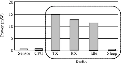
Energy consumption of node subsystems is shown in
Figure 2 [7]. There are four possible states for sensor node’s radio to select: transmit, receive, idle, or sleep. It is obtained that the: Energy Consumption of Sensor Node’s radio component is:
TX RX IDLE SL
E
≈
E
≈
E
>>
E
Thus, it is judicious to completely shut down the radio when it is not transmitting or receiving data in order to keep power.
2.2. Clustering of Sensor Nodes
Sensor nodes in WSN can be divided into some groups called clusters to realize data gather with efficient net-work organization, in which has a cluster head (CH) and a number of member nodes. Clustering produces a two- layer hierarchy in WSN. Cluster heads (CHs) belong to
Sensor ADC
Processing Unit
storage
Transceiver Power Unit
Sensor Unit
[image:2.595.326.522.79.181.2]Processor
Figure 1. The components of a sensor node.
5
0 10 15 20
P
o
w
er (m
W
)
Sensor CPU TX RX Idle Sleep
Radio
Figure 2. Energy consumption of sensor nodes.
the higher layer while member nodes the lower layer. The members of a cluster can communicate with their CH directly. A CH can forward the fused data to the cen-tral base station through other CHs.
The member nodes send their data to the respective CHs. Then the CHs fuse the data and transmitted them to the base station through other CHs. CHs may lose more energy because of transmitting data over longer dis-tances.
2.3. Duty Cycling
Duty cycling is very important in wireless sensor for conserving energy, which makes the radio transceiver be in the sleep mode while communication is not required. Thus, sensor nodes change between active and sleep state based on network activity, which is known as duty cycl-ing. Duty is cycling defined as time slots that nodes are active during their lifetime. For target tracking, since sensor nodes perform a task cooperatively, it is necessary to coordinate their sleep/wakeup times. A sleep/wakeup scheduling algorithm is employed to decide state trans-formation (active to sleep and vice versa) of sensor nodes.
3. Deployment of Sensor Nodes
Different shapes to forming node into clusters have been proposed for deploying nodes, such as circle, quadrila-teral, and hexagon. The honeycomb is often used be-cause it corresponds to the shape of the radio transmis-sion range, which may result in overlapping between clusters or uncovered areas. The hexagon is an ideal shape for clustering a large area into adjacent, no over-lapping areas, which can be proved as follows.
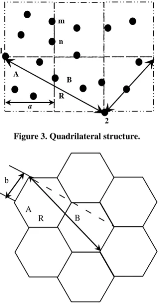
Quadrilateral structure for parting sensing region is shown in Figure 3, in which nodes are divided into small cluster. The clusters are defined as that two neighboring clusters A and B, where all nodes in A can communicate with all nodes in B and vice versa.
[image:2.595.60.286.602.704.2]on marked value in Figure 3, functions can be expressed as follow:
( )
22 2
2
a + a ≤R (1)
2 2
2a =r (2)
5
a≤R (3) Honeycomb structure for parting sensing region is shown in Figure 4; functions can be expressed based on marked value in Figure 4.
(
)
22 2
2 3
b + b ≤R (4)
13
b≤R (5) Thus, area of quadrilateral and each honeycomb can be expressed by:
2 2 2
5 0.2 q
S =a =R = R (6)
2 3 3 2 2
3sin 60 0.2
26 h
S = ° =b R ≈ R (7)
Note that the one-hop coverage area of quadrilateral structure is Sqc= 5Sq = R2 andthe one-hop coverage area of honeycomb structure forwarding is Shc = 7 Sh≈ 1.4R2, so the one-hop coverage area of honeycomb structure is about 40% larger than that of quadrilateral structure.
2 m
n
a 1
A
[image:3.595.93.259.397.708.2]B R
Figure 3. Quadrilateral structure.
R b
B A
Figure 4. Honeycomb structure.
4. Sensor Scheduling During Target Moving
4.1. Dynamic Clustering
Dynamic cluster architectures means that clusters will be formed with certain events of interest coming, such as target appear. If a sensor node with sufficient energy and computational power detects signals of interest, it would be selected as a CH (cluster head). Sensors near to the active CH are invited to join the cluster and send their information to the CH.
At any time instant only one cluster is active with tar-get moving, in which sensors nodes are in the active state and all other sensors are shut down (Figure 5) Sensor scheduling mechanism properly adapt to a scalable and dynamic network topology. The network activity can be set in time slots. Then, active sensor nodes are selected at the beginning of time slot corresponding to trajectory of target. Active node selection is chosen according to the connectivity, power efficiency and so on.
Sensor scheduling problem is employed to select sen-sors to form cluster dynamically in order to optimize the tracking performance of the targets. The sensor nodes being activated at time ti must be chosen at or before
time ti − TK, where TK is the time needed to select and activate a sensor cluster.
4.2. Maximum Entropy Clustering
The objective of a clustering algorithm is the assignment of a set of M feature vectors xi∈ X into k clusters,
which are represented by the prototypes cj ∈ C. The certainty of the assignment of the feature vectors xi ∈ X
into various clusters is measured by the membership
functions uij [0, l], j = 1, 2, k, ( 1 i
ij iju =
∑
).For a given set of membership functions, the distortion between the feature vectors xi ∈X and the prototypes cj ∈ C is measured by[13-15].
(
)
1 1(
)
1
, M k ,
ij i i j ij i j
D u U c C u d x c
M = =
∈ ∈ =
∑ ∑
(8)cluster
sensor node moving target
active
[image:3.595.320.539.557.704.2]where d (xi, cj) is a metric of the distance between the
feature vector xi ∈ X and the prototype cj∈C,
(
)
2i i i i
d x −c = x −c (9)
In the maximum uncertainty or minimum selectivity phase, the clustering process is based on the minimiza-tion of the negative entropy, given by
(
)
1 1* ij Mi kj ijlog ij
E u ∈U =
∑ ∑
= =u u (10)Assume that the sensor network including k numbers of sensor nodes can be divided into M numbers of clus-ters, and the matrix of cluster head is
{
1 2}
H= H , H ,, Hz and uij is the degree of
member-ship of node xi in cluster j.
(
)
21 1 1 1
1
, log
ij
M k M k
ij ij ij
i j i j
I u H u d u u
λ
= = = =
=
∑∑
+∑∑
(11)( )1
1
ij ij
c
d d
l ij
k
u + e−λ e−λ
=
=
∑
(12)( )1 ( )1 ( )1
1 1
k k
l l l
i ij j ij
j j
H + u + x u +
= =
=
∑
∑
(13)The Clustering process is described as follows: 1) Initialization of cluster head is assumed as
( )0
{
( )0 ( )0 ( )0}
1 , 2 , , c
H = H H H
2) Defining convergence threshold ε
3) Updating uij and cluster head with expressions (12)
and (13) until
( ) ( )
(
1)
max Hil Hil ε
+ − <
4.3. Predication of Trajectory
During the target tracking, when to wakeup sensor nodes to form cluster for performing tracking task is mainly based on the location of target in next time slot. Thus, it is necessary to estimate precisely the trajectory of targets. In this paper, we use Kalman filter to predict the trajec-tories of target. The Kalman filter is a set of mathemati-cal equations that is efficient to estimate the state of a process, because it supports estimations of past, present, and even future states.
The Kalman filter estimates a process using feedback control, so the equations for the Kalman filter include time update equations and measurement update equa-tions. The time update equations represent projecting forward the current state and error covariance estimates to achieve the a priori estimates for the next time step [16].
The state vectors of all targets at time tkis expressed
by xk = x xk1, k2,,xkn, where i k
x is the state vector of
target i and n represents the number of targets. The state equation of the n targets is set by
1 1
k k k
X = ⋅A X − +W− (14)
with a measurement that is
k k k
Z =H +V (15)
The random variables Wkand Vk represent the process
and measurement noise (respectively).They are assumed to be independent (of each other), white, and with normal probability distributions
Where A is a linear function, and Wk is independent
white noise. Five basic equations of Kalman filter (time update equations, measurement update equations) is given by [16]
(
1)
(
1 1)
( )
X k k− = ⋅A X k− k− +W k (16)
(
1)
1)(
1 1)
TP k k− = ⋅A P k− = ⋅A P k− k− A +Q (17)
( )
(
1)
g( ) ( )
(
(
1)
)
X k k =X k k− +K k Z k − ⋅H X k k− (18)
(
)
'(
(
)
)
1 1 T
g
K =P k k− ⋅H H P k k⋅ − H +R (19)
( )
(
g( )
)
(
1)
P k k = I−K k ⋅H P k k− (20)
The process is repeated with the previous a posteriori estimates used to predict the new a priori estimates with each time and measurement update.
4.4. Sensor Scheduling
When a target appears in the sensor network, it can be sensed when sensor nodes’ detected signal strength beyond a predefined value. Then, sensor nodes are se-lected to form a cluster dynamically. There are a cluster head and several member nodes in each cluster. The sensor information is passed on to cluster heads where, in turn, transmit information to the base station.
With the target moving, different sensor nodes are chosen to form another cluster and the nodes in this cluster are awakened while make other sensor nodes be in sleep mode based on the prediction of trajectory of target and node’ energy and location. Thus, it is possible to save energy during tracking with duty cycling and cluster technology.
5. Conclusions
that perform tasks be in the active state and all other sensors are in the sleep state. In later research, we will attempt to study follows problem: 1) how to determine each node whether to enter sleep mode? 2) How long should a sensor be in the sleep state?
6. References
[1] J. Kahn, R. H. Katz and K. Pester, “Next Century Chal-lenges: Mobile Networking for Smart Dust,” ACM MO-BICOM Conference, 1999.
[2] F. Zhao, J. Liu, J. Liu, L. Guibas and J. Reich, “Collabor-ative Signal and Information Processing: An Informa-tion-Directed Approach,” Proceedings of the IEEE,
200
[3] V. Raghunathan, C. Schurgers, S. Park and M. B. Srivast- ava, “Energy-Aware Wireless Microsensor Networks,” Signal Processing Magazine IEEE, Vol. 19, No. 2, 2002,
pp. 40-50.
[4] D. M. Blough and P. Santi, “Investigating Upper Bounds on Network Lifetime Extension for Cell-Based Energy Conservation Techniques in Stationary ad hoc NetWork,” Proceeding of 8th Annual International Conference on Mobile Computing and Networking, GA, USA, ACM Press, Atlanta, 2002, pp. 183-192.
[5] Y. Xu, J. Heidemann and D. Estrin “Geography-Informed Energy Conservation for ad hoc Routing,” Proceedings Annual International Conference Mobile Mobicom, 2001, pp. 70-84.
[6] J. Y. Lin, W. D. Xiao, F. L. Lewis and L. H. Xie, “Ener-gy-Efficient Distributed Adaptive Multisensor Schedul-ing for Target TrackSchedul-ing in Wireless Sensor Networks,” IEEE Transactions on Instrumentation and Measurement, Vol. 58, No. 6, 2009, pp. 1886-1896.
[7] D. Estrin, “Wireless Sensor Networks Tutorial Part Iv: Sensor Network Protocols,” In Preceding Mobicom, USA, pp. 23-28, 2002.
[8] T. Ratnasingham, K. Thiagalingam, L. Marcel and
Her-nandez, “Large-Scale Optimal Sensor Array Management for Multitarget Tracking, IEEE Transactions on Systems, Man and Cybernetics—Part C: Applications and Reviews, Vol. 37, No. 5, 2007, pp. 803-814.
[9] M. Cardei, M. T. Thai and Y. S. Li, et al. “Energy-Efficient Target Coverage in Wireless Sensor Networks,” Pro-ceedingsof IEEE INFOCOM, 2005, Vol. 42, No. 3, pp.
1976-1984
[10] I. F. Akyildiz, W. S. Y. Sankarasubramaniam and E. Cayirci, “Wireless Sensor Networks: a Survey,” Com-puter Networks, Vol. 38, No. 4, 2002, pp. 393-422.
[11] A. Giuseppe, C. Marco, D. F. Mario and P. Andrea, “Energy Conservation in Wireless Sensor Networks: A Survey,” Ad Hoc Networks, 2009.
doi:10.1016/S1389-1286(01)00302-4
[12] Z. Wang and J. Zhang, “Energy Efficiency of Two Vir-tual Infrastructures for MNAETs,” IPCCCC, Vol. 42, No.
3, 2006, pp. 547-552.
[13] D. M. Yan, J. K. Wang, L. Liu, B. Wang and P. Xu, “Topology Control Algorithm Target Track-ing-Oriented,” The 5th International Conference on Wireless Communications, Networking and Mobile Computing, Vol. 4, 2009, pp. 1-4.
doi:10.1109/WICOM.2009.5304199
[14] N. B. Karayiannis, “MECA: Maximum Entropy Cluster-ing Algorithm,” Proceedings of the Third IEEE Confe-rence on Fuzzy Systems, IEEE World Congress on Com-putational Intelligence, Vol. 1, 1994, pp. 630-635.
[15] X. Wang, S. Wang and A. Jiang, “A Novel Framework for Clusterbased Sensor Fusion,” IMACS Multiconference on Computational Engineering in Systems Applications, Vol. 2, 2006, pp. 2033-2038.