http://www.scirp.org/journal/wsn ISSN Online: 1945-3086 ISSN Print: 1945-3078
A Novel Cluster Based Time Synchronization
Technique for Wireless Sensor Networks
Gopal Chand Gautam, Narottam Chand
Department of Computer Science & Engineering, National Institute of Technology Hamirpur, Hamirpur, India
Abstract
Time synchronization is one of the important aspects in wireless sensor net-works. Time synchronization assures that all the sensor nodes in wireless sensor network have the same clock time. There are various applications such as seismic study, military applications, pollution monitoring where sensor nodes require synchronized time. Time synchronization is mandatory for many wireless sensor networks protocols such as MAC protocols and also important for TDMA scheduling for proper duty cycle coordination. Time synchronization is a stimulating problem in wireless sensor networks because each node has its own local clock which keeps on varying due to variation in the oscillator frequency. The oscillator frequency is time varying due to am-bient conditions which leads to re-synchronization of nodes time and again. This re-synchronization process is energy consuming whereas energy is con-straints in WSN. This paper proposes a novel cluster based time synchroniza-tion technique for wireless sensor networks in which cluster head rotasynchroniza-tion is based on minimum clock offset. Simulation results based on energy analysis of the proposed model demonstrate that proposed novel cluster based time synchronization technique reduces the energy consumption and also the syn-chronization error compared with other existing protocols.
Keywords
Cluster, Offset, Delay, Time Synchronization
1. Introduction
Recent advancements in the electronic and communication technologies have resulted in the emergence of wireless sensor networks (WSNs). WSNs are com-posed of small size, low power and low cost wireless micro-sensors, known as Sensor Nodes (SNs) [1][2][3]. These SNs can be embedded in various objects in order to form intelligent multipurpose distributed systems. These SNs generally How to cite this paper: Gautam, G.C. and
Chand, N. (2017) A Novel Cluster Based Time Synchronization Technique for Wire-less Sensor Networks. Wireless Sensor Net-work, 9, 145-165.
https://doi.org/10.4236/wsn.2017.95008
Received: May 1, 2017 Accepted: May 22, 2017 Published: May 25, 2017
Copyright © 2017 by authors and Scientific Research Publishing Inc. This work is licensed under the Creative Commons Attribution International License (CC BY 4.0).
perform three major tasks i.e. sensing, data processing and communication [4]. SNs are capable of sensing various environmental conditions such as sound, temperature, humidity, strain, acidity pressure, vibration, motion or pollutants [5][6], etc.
Wireless Sensor Network (WSN) consists of large number of SNs deployed in unattended environment [7]. These SNs monitor objects in the sensing field and report the activities and events to sink. In order to establish correct logical order of the events, the data must be time stamped by the SNs. In WSN some applica-tions such as military applicaapplica-tions require accurate time of the event. Data fu-sion in WSN also demands time stamp of SNs to suppress the duplicate infor-mation of the SNs. Time is also important to implement the TDMA schedule in WSNs. Due to various challenges and constraints in WSNs, the clock synchro-nization protocols (NTP) [8][9] designed by researchers for wired networks do not work in wireless sensor networks. In WSNs each node has its own local clock that may vary from the local clock of other nodes in the network which leads to clock offset. Higher clock offset degrade the WSNs performance and the infor-mation collected by the nodes may not provide the accurate timing of the event. Whereas time synchronization in WSNs is important for efficient duty cycling, location based monitoring, target/event tracking data fusion and network sched-uling and routing.
Keeping in view the importance of time synchronization as well as the con-straints of SNs, the objective of the proposed research is to develop time syn-chronization technique that helps to synchronize the SNs in an energy efficient manner. This paper proposes a novel cluster based time synchronization tech-nique for wireless sensor networks to keep local clocks of all the SNs synchro-nized with global clock.
In wireless sensor networks, a lot of research [10]-[31] has already been car-ried out to design time synchronization protocols such as Reference Broadcast Synchronization (RBS) [11], Romer synchronization [13], TPSN (Timing Sync Protocols for Sensors Networks) [15], Two-hop time synchronization protocol for sensor networks (TTS) [18], Fast distributed multi-hop relative time syn-chronization protocol and estimators for wireless sensor networks [19], Long term and large scale time synchronization in wireless sensor networks (2LTSP) [20], and Average time synchronization in wireless sensor networks by pairwise messages (ATSP) [21], Time synchronization protocol based on spanning tree [28], Lightweight and Energy Efficient Time Synchronization (LEETS) Protocols [29] and Lightweight Fault-tolerant Time synchronization [30]. Some of these protocols synchronize the nodes internally by placing the nodes on common no-tion of time and some synchronize externally by using large number of messages to adjust the clocks of the sensor nodes with global clock.
(EECA) and then time synchronization is performed.
The rest of the paper is organized as follows. In Section 2 describes the pro-posed energy efficient clustering algorithm (EECA) for WSNs. Section 3 de-scribes the proposed time synchronization algorithm and synchronization error estimation. Energy analysis is performed in Section 4. Section 5 contains simula-tion and analysis and finally we conclude the paper in Secsimula-tion 6.
2. Energy Efficient Clustering Algorithm
In this section, we describe our proposed protocol, called Energy Efficient Clus-tering Algorithm (EECA) for wireless sensor networks. The proposed technique has been segregated into different phases; creation of clusters to prolong the network lifetime, CH selection and cluster head rotation. EECA forms clusters before selecting cluster-head. Our proposed EECA works in three steps: (2.1) Cluster formation process, (2.2) Cluster head selection process and (2.3) Cluster head rotation process.
2.1. Cluster Formation Process
In EECA clustering process is initiated by the sink. Sink calculates the prelimi-nary mean points by sensing field size, optimum number of clusters and average distance of the nodes from the center of the sensing field. After the deployment of SNs in sensing field, the sink initiates the clustering process by finding the centroid of the sensing field by using the Equation (1) where
2
i i
L x = and
2
i i
B
y = where Li and Bi is the size of the sensor field and Ai is the area of
the sensing field.
(
)
Centroid , where i i and i i
i i
y A x A
x y x y
A A
= =
∑
=∑
∑
∑
(1)When the value of centroid is calculated, sink node finds the average distance
d between centroid and all the SNs by using the Equation (2). Where Xi and Yi
are the coordinates of the node SNi.
1 , 1
n n
i i
i X x i Y y
d
n n
= =
− −
=
∑
∑
(2)Sink also computes the optimum number of clusters k using the Equation (3) [32]. The total number of nodes deployed in the sensing field is n, M is the side of square sensing field and dto BS is average distance to cluster heads from the
base station. εfs is energy coefficient of power amplifier stage of SN for free space energy dissipation model and εmp is energy coefficient of power amplifier stage of SN for multipath energy dissipation model.
2π
fs
mp to BS
n M
k
d
ε ε
= (3)
the preliminary mean points
(
,)
x yj j j
M m m where j=1, 2,,k using Equa-tion (4) and broadcasts the locaEqua-tions of preliminary mean points to the SNs.
(
)
(
)
2π
cos 1
2π
sin 1
x
y
j
j
m d j x
k
m d j y
k
= × × − +
= × × − +
(4)
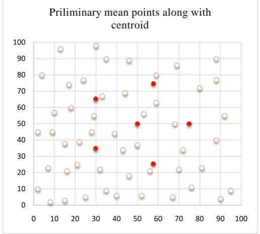
The objective of finding the preliminary mean points is to significantly reduce the iteration time of cluster formation. Figure 1 shows the preliminary mean points in 100 m × 100 m sensing filed area with 50 sensor nodes.
When the SNs receive the sink message of preliminary mean points, each node find its minimum distance from preliminary mean points by using the Eq-uation (5) and retain the minimum distance.
2
1
Arg.Min
i j
k
i j
j= X∈C X −m
∑ ∑
(5)i
X is the coordinate of SNi, Cj is the cluster j and mj is the coordinate of preliminary mean points. The minimum distance between preliminary mean points and SNs helps to form uniform distributed clusters. Nodes join the cluster on the minimum distance to the preliminary mean points using the Equation (6). In each round SNs check their distance with all nearby clusters and node nearest to the preliminary mean point mj in the r
th round joins the cluster j.
( ) ( ) ( )
*
2 2
*
: for all 1, 2, ,
r r r
j i i j i j
C =X X −m ≤ X −m j = k
(6)
( )r j
[image:4.595.244.503.470.702.2]C is the Cluster j in rth round. After tagging all the nodes with different clusters new mean points are created by using the Equation (7).
Figure 1. Preliminary mean points along with centroid where n = 50
and k = 5. 0 10 20 30 40 50 60 70 80 90 100
0 10 20 30 40 50 60 70 80 90 100
( )
( ) ( )
1 1
r j j
r
j r X C j
j
m X
C +
∈
=
∑
(7)( )r j
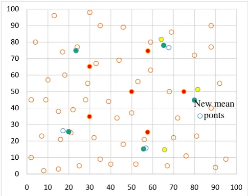
C is the number of SNs in the cluster j. Figure 2 shows the new mean points.
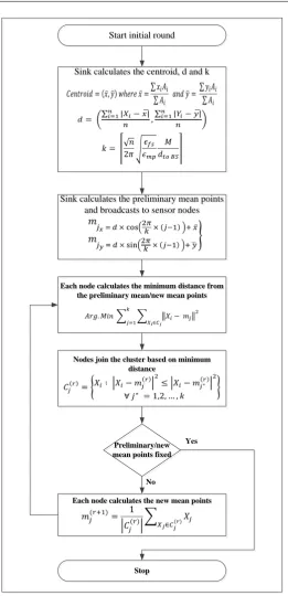
The process of finding the new mean points is iterative till the new mean points stop moving. As long as the preliminary mean points keep on changing the nodes are re-arranged again and again as per the Equation (6) and (7). The cluster formation process is complete when the new mean points are fixed and nodes join the final mean points with minimum distance. Figure 3 shows the flowchart of clustering process.
2.2. Cluster Head Selection
The clustering algorithm divides the whole network into different clusters. The next step is to elect CH within each cluster. Each node within the cluster calcu-lates its distance from the cluster by using the Equation (8). Where Xi is the
coordinates of the SNi and Cj is the coordinates of the final mean point in which
the SNi tagged itself.
i i j
D = X −C (8) The cluster head selection is performed using back off timer strategy. SNi sets
its back off timer by using the Equation (9).
average
Counter i
i i
D RV D
= ∗ (9)
i
RV is the random variable between [0.9, 1]. Di is distance of SNi from final
mean point in a cluster. Daverage is average distance of all the senor nodes within a cluster.
[image:5.595.246.500.503.703.2]The back off timer of each node starts decrementing and the node whose back
Figure 2. New mean points after three iterations where n = 50 and k = 5.
0 10 20 30 40 50 60 70 80 90 100
0 10 20 30 40 50 60 70 80 90 100 New mean
Start initial round
Start initial round
Sink calculates the centroid, d and k
Sink calculates the centroid, d and k
Sink calculates the preliminary mean points and broadcasts to sensor nodes
Sink calculates the preliminary mean points and broadcasts to sensor nodes
Each node calculates the minimum distance from the preliminary mean/new mean points Each node calculates the minimum distance from
the preliminary mean/new mean points
Preliminary/new mean points fixed Preliminary/new mean points fixed
Nodes join the cluster based on minimum distance
Nodes join the cluster based on minimum distance
Each node calculates the new mean points Each node calculates the new mean points
Stop Stop
Yes
[image:6.595.243.505.56.598.2]No
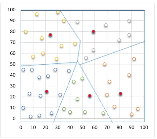
Figure 3. Flowchart of clustering process.
Figure 4. Clustering with CH where n = 50, M = 100 m and k = 5.
2.3. Cluster Head Rotation
The role of CH in a cluster must be rotated regularly among its members to prolong the network lifetime of sensor network by balancing the energy con-sumption of various sensor nodes. CH is required to perform extra tasks such as data gathering, data aggregation, etc. compared to the other sensor nodes. Ener-gy consumption of CH is more compared to other sensor nodes therefore, some mechanism must be applied for CH rotation among the cluster members. A number of methods for CH rotation have been discussed in literature [33]-[38].
In CH rotation process, the new CH is selected from cluster members. CH ro-tation/re-election process is initiated when residual energy of a node falls below the threshold value. The new CH is elected with higher value of Candidacy fac-tor (CF). Candidacy facfac-tor of SNi is defined as
i Resi i
i i
E CF
D θ
=
× (10)
where i Resi
E is residual energy of SNi, Di is the distance between SNi and
cen-troid of the cluster. θi is clock offset of SNi. Each node sends its CFi value to
cluster head. CH would choose the node with highest CFi value and pass
in-formation to sink and other members about new cluster head. Figure 5 shows the flowchart of CH selection/rotation process.
3. Cluster Based Time Synchronization
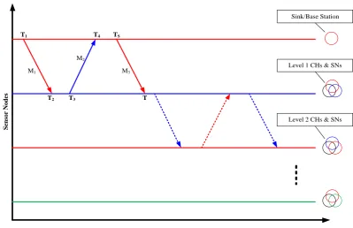
The proposed cluster based time synchronization (CBTS) algorithm is based on external synchronization. Once the clustering process is complete using EECA protocol proposed in section 3, time synchronization process is initiated by the parent node, which is the sink/base station during the initial phase. Sink/base station is used as a reference node for time. The proposed algorithm is using k
0 10 20 30 40 50 60 70 80 90 100
CHs. There are k' CHs at level-1 and k'' CHs at level-2. The proposed model is shown in Figure 6.
Start cluster head election and rotation process
Start cluster head election and rotation process
Each node calculates the Di
Each node calculates the Di
Calculate the value of Counteri and
select the nodes with least value Calculate the value of Counteri and
select the nodes with least value
Within a cluster calculate the value
of CFi for each node and select a
node with maximum CFi as CH
Within a cluster calculate the value of CFi for each node and select a
node with maximum CFi as CH
Stop Stop Cluster head
election/ rotation Cluster head
election/ rotation
[image:8.595.238.509.116.407.2]Election Rotation
Figure 5. Flowchart for selection and rotation of cluster head.
Time
Sensor Nodes
T1 T4
T2 T3
TS
T
Sink/Base Station
Level 1 CHs & SNs
Level 2 CHs & SNs M1
M2
M3
[image:8.595.137.537.446.704.2]The parent node (Pn) initiates the synchronization process by broadcasting
the Syn_start packet which contains the timestamp T1 and then waits for the
reply. When the CHs of level 1 (CHL1) receive Syn_start packet, they send reply
to sink/base station by sending the Syn_ack packet. The Syn_ack packet contains the timestamp T T T1, 2, 3 where time T1 is the time of sending Syn_start packet,
2
T is the time when the CHs of level 1 receive the packet and T3 time when
CHs of level 1 send the Syn_ack packet. The parent node after receiving the
Syn_ack packets, broadcasts Syn_pkt with timestamp T T T T T1, 2, 3, 4, s where T4
is the time when the parent node receives the Syn_ack packet and Ts is the time
to set the clocks of the CHs of level-1. All CHs of level-1 receive the Syn_pkt and calculate the offset (θ) and delay (δ) and set the clocks as:
s
T=T + ±θ δ (11) In the initial synchronization phase, sink/base station functions as parent node. After synchronizing the CHs of level 1, it further functions as parent nodes and synchronizes the cluster nodes and CHs of level 2. Cluster based time syn-chronization algorithm is as below:
Sink/Base Station
1. Tm = +t tα
2. while nodes are not synchronized do
3. set SCOUNT = k' × Tm
4. Pn broadcasts (Syn_start, T1)
SCOUNT - -
5. if Pn wait for reply && SCOUNT = = 0 then repeat step 4
6. else
n
P receive (Syn_ack, T T T1, 2, 3)
7. Pn broadcasts (Syn_Pkt, T T T T T1, 2, 3, 4, s) to CHL1 8. endif
Cluster Heads
9. if CHL1 receives (Syn_start, T1) then send (Syn_ack, T T T1, 2, 3) to Pn
10.else
CHL1 waits
11.endif
12.if CHL1 receives (Syn_Pkt, T T T T T1, 2, 3, 4, s) from Pn then
calculate
δ
=(
T2−T1)
+(
T4−T3)
2calculate
θ
=(
T2−T1)
−(
T4−T3)
2synchronize T =Ts+ ±θ δ
13.else
14.CHL1 waits
15.endif
16.Repeat step from 1 to 15 in next Synchronization Phase
In the algorithms, Tm is the maximum time required to receive a message
from CH and Pn, or vice versa, whereas t is the current time and tαis the
Synchronization Error
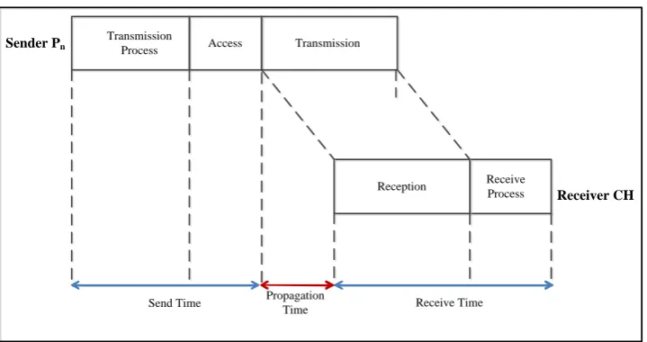
[image:10.595.178.538.523.713.2]All WSN synchronization schemes [10]-[31] have four basic packet delay com-ponents: send time, access time, propagation time, and receive time as shown in Figure 7. The send time is that of the sender constructing the time message to transmit on the network. The access time is that of the MAC layer delay in ac-cessing the network. The time for the bits to be physically transmitted on the medium is considered the propagation time. Finally, the receive time is the time spent by the receiver for processing the message. The synchronization error is calculated by using the time stamp message shown in the Figure 6. In synchro-nization error calculation, access time is combined with send time. The main problem of time synchronization besides having a packet delay is that, it is able to foresee the time spent on each, which can be challenging. Disregarding any of these will significantly surge the performance of the synchronization technique.
In the proposed CBTS synchronization, a message from the sink to SNs transmits through multi-hops that induce the time delay error because of vari-ous delays as shown in Figure 7. Exchange of timestamp messages among parent node and cluster heads (shown in the Figure 6) are used to analyse the synchro-nization error of the proposed CBTS. Simply by using send time, propagation time, receive time and clock drift and then equating the timestamps of cluster head and parent node following equations obtained:
1 1 1 1
2 1
i i i i i i i i
T + =T +α +δ→ + +β+ +γ→ + (12)
1 1 1 1 1
4 3
i i i i i i i
T =T+ +α + +δ + → +β −γ → + (13)
1 2
i
T+ and T4i represent the timestamps of cluster head and parent node re-spectively, where i=1, 2,, n is representing the level. α β, and δ represent the send time, receive time and propagation delay, respectively. γ is the clock drift of the node. To calculate one-hop synchronization error ωi→ +i1 subtract
the Equation (12) from Equation (13) as:
1 1 1 1 1 1 1 1 1
2 4 1 3 2
i i i i i i i i i i i i i i i
T+ −T =T −T+ +α −α + +δ → + −δ+ → +β+ −β +γ → + + γ → +(14)
Sender Pn
Receiver CH
Transmission
Process Access Transmission
Reception Receive
Process
Send Time Propagation
Time Receive Time
Dividing both sides by 2
(
1) (
1)
1 1 1 1 12 1 4 3 1
2 2 2 2
i i i i i i i i i i i
i i
T T T T α α δ δ β β
γ
+ + + → + + → +
→ +
− − − − − −
− = + + (15)
1 1 1 1 1
1 1
2 2 2
i i i i i i i
i i i i α α δ δ β β
θ→ + −γ → + = − + + → + − + → + + − (16)
where Offset θi→ +i1 is computed as 1
(
1) (
1)
2 1 4 3 2
i i i i i i
T T T T
θ
→ + = + − − − + and
by subtracting the clock drift from the clock offset, synchronization error for one-hop ωi→ +i1 is obtained as:
1 1 1 1 1
1
2 2 2
i i i i i i i
i i
α α δ δ β β
ω→ + = − + + → + − + → + + − (17)
The Equation (17) can be modified to obtain multi-hop synchronization error as:
1 1 2 1 1 1 1 2 2 1
1 2 1
2 2 2 2
2 2
i i i i i i i i i i i
i
i i i
α α α α δ δ δ δ
ω
β β β β
+ + + → + + → + → + + → + + + − − − − = + + + + − − + + + + (18)
(
1) (
1 1 1) (
1)
1
1
2
l i i i i i i i
i i
ω
α α
+δ
→ +δ
+ →β
+β
=
=
∑
− + − + − (19)Equation (19) calculates synchronization error for multi-hop communication. The objective of finding the synchronization error ωi is to ensure that at any
real time T, ωi is between lower and upper bounds
[
min , maxε ε]
. If the valueof synchronization error goes below minε or exceeds maxε, the
resynchro-nization process is initiated by the sink/base station.
4. Energy Analysis of CBTS
Energy analyses of CBTS algorithm is performed for l levels of CHs by using the energy models [32][39][40][41][42]. Since most of the energy is dissipated by the SNs in communication, therefore the energy analysis is performed for the transmission and reception of m bit message for a distance of d. To transmit m
bit message over a distance d, the energy cost of transmission
( )
ETx is as:(
)
2 04 0 if , if elec fs Tx elec mp
m E m d d d
E m d
m E m d d d
ε
ε
∗ + ∗ ∗ ≤
=
∗ + ∗ ∗ >
(20)
elec
E is the energy dissipation per bit to run transmitter and receiver elec-tronics circuitry. εfs is the energy coefficient of power amplifier stage of sensor nodes for free space energy dissipation model when transmission distance is less than threshold i.e. d<d0. εmp is the energy coefficient of power amplifier stage of sensor nodes for multipath energy dissipation model when transmission distance is greater than threshold i.e. d≥d0. For d=d0, distance threshold
can be calculated as d0 =
ε ε
fs mp.The energy consumed to receive m bit data is expressed as:
Rx elec
Initially two-level network is considered, where Total number of nodes = n
Total number of cluster heads = k
Number of level 1 CHs = k'
Number of level 2 CHs = k''
Number of normal sensor nodes = n − k
The proposed CBTS algorithm uses n+2
(
k+1)
messages to synchronize n number of SNs. The energy dissipation for receiving and transmitting m bit time synchronization message derived below depends on the number of messages re-ceived and transmitted by the SNs. As the sink/base station is at level 0 with no constraint of energy, the energy exhausted during transmitting and receiving mbit time synchronization message at level 1 CHs and level 2 CHs is calculated by using the Equations (20) and (21).
Energy consumption at level 1 CHs: Total energy consumed in CBTS pro-tocol while receiving and sending synchronization messages at level 1 CHs is given by Equation (22) and (23)
(
ERx,1,ETx,1)
respectively and the total energyconsumed at level 1 CHs is given by Equation (24)
(
ETotal,1)
.,1 3
Rx elect
E = k mE′ (22)
2 4
,1 2
π
Tx elect mp n elect fs
M
E mE m d toP k mE m
k
ε ′ ε
= + + +
′′
(23)
2 4
,1 3 2
π
Total elect elect mp n elect fs
M
E k mE mE m d to P k mE m
k
ε ε
′ ′
= + + + +
′′
(24)
Energy consumption at level 2 CHs: Energy consumed by level 2 CHs while receiving and transmitting synchronization messages is given by Equations (25) and (26)
(
ERx,2,ETx,2)
respectively and the total energy consumed by level 2CHs is given by Equation (27)
(
ETotal,2)
.,2 3 .
Rx elect
E = k mE′′ . (25)
(
)
2 2
,2 2 .
π π
Tx elect fs elect fs
M M
E k mE m k mE m
k N k
ε ε
′ ′′
= + + +
′ −
(26)
(
)
2 2
,?2 3 π 2 π .
Total elect elect fs elect fs
M M
E k mE k mE m k mE m
k N k
ε ε
′′ ′ ′′
= + + ′+ + −
(27)
Energy consumption at SNs level: Energy consumed by SNs while receiving and sending synchronization messages is given by Equations (28) and (29)
(
ERx sensor, ,ETx sensor,)
respectively and the total energy consumed by SNs for re-ceiving and sending time synchronization messages is given by Equation (30)(
ETotal sensor,)
.(
)
, 2
Rx sensor elect
E = n−k mE (28)
2
, π
Tx sensor elect fs
M
E k mE m
k ε ′′ = + ′′
(29)
(
)
2, 2
π
Total sensor elect elect fs
M
E n k mE k mE m
k ε ′′ = − + + ′′
Total energy consumption for communication: The energy consumption rate for sensors in a WSN contrasts significantly on the basis of the protocols the sensors employ for communications. However, the total energy expended for communication of synchronization messages in the proposed model is given by Equation (31) which is further simplified in Equations (32)-(39). Therefore, the total energy dissipation for a single round of time synchronization for l level of hierarchical sensor networks is given by Equation (39).
(
)
(
)
2 4 2 2 2 3 2 π 3 2 π π 2 πGrand Total elect elect mp n elect fs
elect elect fs elect fs
elect elect fs
M
E k mE mE m d toP k mE m
k
M M
k mE k mE m k mE m
k N k
M
n k mE k mE m
k ε ε ε ε ε ′ ′ = + + + + ′′ ′′ ′ ′′ + + + + + ′ − ′′ + − + + ′′ (31)
(
)
2 4 2 2 23 2 2
π
3 2 2
π π
2 2
π
elect elect mp n elect fs
elect elect fs elect fs
elect elect elect fs
M
k mE mE m d toP k mE k m
k
M M
k mE k mE k m k mE k m
k n k
M
nmE kmE k mE k m
k ε ε ε ε ε ′ ′ ′ = + + + + ′′ ′′ ′ ′ ′′ ′′ + + + + + ′ − ′′ ′′ + − + + ′′ (32)
(
)
2 2 2
2
4
3 2 3 2
2 2
π π π
2 2
π
elect elect elect elect elect elect
elect elect fs fs fs
fs mp n elect
k mE k mE k mE k mE k mE k mE
M M M
nmE mE k m k m k m
k k k
M
k m m d toP k mE
n k
ε ε ε
ε ε ′ ′ ′ ′′ ′′ ′′ = + + + + + ′ ′ ′′ + + + + + ′′ ′ ′′ ′′ ′ + + + − (33)
Solving above, following equation is obtained:
(
)
(
)
2 2 2
4
3 2 3 2 2 2
2
2 2
π π
elect elect elect elect
fs fs fs mp n
k k k k k k mE kmE nmE mE
k M M M
m m k m m d toP
k ε π ε ε n k ε
′ ′ ′ ′′ ′′ ′′ = + + + + + − + + ′ ′′ + + + + ′′ − (34)
(
)
(
)
2 46 2 2
2 2
2
π
elect elect elect elect
fs mp n
k k mE kmE nmE mE
k k M
m m d toP
n k k ε ε
′ ′′ = + − + + ′′ ′ + − + ′′ + + (35)
(
)
2 4 2 24 2 2
π
elect elect elect fs mp n
k k M
kmE nmE mE m m d toP
n k k ε ε
′′ ′
= + + + − + ′′ + +
(36)
(
)
(
2)
2 2 44 2 1 2
π
elect fs mp n
k k M
k n mE m m d toP
n k k ε ε
′′ ′
= + + + + + +
′′ −
(37)
(
)
(
)
1 2 42
4 2 1 2 1
π
i i
n
elect i i fs mp n
k k M
k n mE m m d toP
n k k ε ε
− = = + + + + + + −
∑
(38)Equation for l Level (i > 2) can be standardized as:
(
)
(
)
1 2 4, 4 2 1 2 1 π
i i
l
total i elect i i fs mp n
k k M
E k n mE i m m d toP
n k k ε ε
where the value of 2 toCH
d is taken as
2
π M
k and the value of
4 n
d toP can be ob- tained as:
(
)
(
)
42
4
2
0 d d .
n Pn
Pn
P y M x x
n y x x M
x y y
d toP x y
M
= −
= − −
+ −
=
∫ ∫
(40)5. Simulation and Results
In this section, the performance of Cluster Based Time Synchronization (CBTS) algorithm has been evaluated through simulation. The simulation has been per-formed in MATLAB 2013a. The performance of CBTS protocol is compared with TPSN [15] and TTS [18] protocols. The performance metrics include the number of nodes in the WSN, initial energy of the SNs, total number of messag-es per synchronization round, total energy dissipation per synchronization round, propagated synchronization error and convergence time. The simulation parameters are listed in Table 1 where for each parameter, simulation has been run many times and the average result of all runs has been taken for evaluation.
The performance evaluation includes message complexity, total energy dissi-pation per synchronization round, propagated synchronization error with num-ber of hops and convergence time.
[image:14.595.207.538.558.732.2]The message complexity in terms of the total number of time synchronization messages per synchronization round while the number of nodes varies from 50 to 500 and the sensing field area is kept constant i.e. 300 m × 300 m as shown in the Figure 8. The simulation results show that the number of time synchroniza-tion messages increase with the increase in the number of nodes in a constant field size because increase in number of nodes leads to increase in time synchro-nization messages. There is a significant reduction in terms of time synchroniza-tion messages in the proposed CBTS method than TPSN and TTS methods. TPSN requires
n n
+
messages to synchronize n SNs and TTS requires n+n 2 messages. CBTS reduces the number of synchronization messages by 40% as compared to TPSN and 25% as compared to TTS. The proposed CBTS methodTable 1. Simulation parameters.
Parameter Default Value Range
Network size (side of square sensor field) 300 m 100 m ~ 500 m
Number of nodes 300 50 ~ 500
Initial energy of node 2 Joule
Sink location (0, 0)
Data packet size (k) 16 KB
Eelec 50 nJ/bit
ɛfs 10 pJ/bit/m2
ɛmp 0.00134 pJ/bit/m4
Data rate 10 Kbps
Number of nodes
50 100 150 200 250 300 350 400 450 500
50 100100 150150 200200 250250 300300 350350 400400 450450 500500
50 100100 150150 200200 250250 300300 350350 400400 450450 500500
50
T
o
ta
l num
b
er
o
f
m
es
sa
ge
s
p
er
s
ync
hr
o
ni
za
tio
n
ro
und
0 100 200 300 400 500 600 700 800 900 1000 1100
[image:15.595.226.522.73.282.2]TPSN TTS CBTS
Figure 8. Variation in time synchronization messages with number of nodes.
provides the best results in comparison with other protocols. Fewer time syn-chronization messages decrease the overhead in terms of communication and thus increase the network lifetime.
Total energy dissipation is calculated as the amount of energy dissipated within the sensor network to perform time synchronization. Figure 9 shows the comparison of simulation results of energy variation for different protocols such as TPSN, TTS and CBTS. The variation in the energy dissipation is studied by varying number of nodes from 50 to 500, while keeping the sensing field size constant as 300 m. It has been observed that the energy dissipation per round increases with increase in the number of nodes. Increased number of nodes leads to increase in the number of time synchronization messages which increases the total routing energy and thus total node energy consumed. The simulation re-sults in Figure 9(a) show that CBTS protocol provides better performance compared to other two protocols. This is due to the less number of synchroniza-tion messages and better clustering technique as compared to TPSN and TTS.
It has been observed that the energy dissipation incessantly increases with the increase in the sensing field size. The distance between the sink and the sensing node increases with the increase in the sensing field size, which increases the transmission energy cost, although the time synchronization messages remain the same. Aforementioned, the performance of cluster based time synchroniza-tion (CBTS) is better than other two protocols due to the reducsynchroniza-tion in the num-ber of synchronization messages and better clustering approach.
Number of nodes
50 100 150 200 250 300 350 400 450 500
50 100100 150150 200200 250250 300300 350350 400400 450450 500500
50 100100 150150 200200 250250 300300 350350 400400 450450 500500
50 T o ta l e ne rgy d is si p at io n p er s ync hr o ni za tio n ro und ( J/ ro und ) 0.00 0.05 0.10 0.15 0.20 0.25 0.30 0.35 0.40 0.45 0.50 0.55 0.60 TPSN TTS CBTS (a)
Sensing field size
100 150 200 250 300 350 400 450 500
100 150 200 250 300 350 400 450 500
100 150 200 250 300 350 400 450 500
100 150 200 250 300 350 400 450 500
100 150 200 250 300 350 400 450 500
[image:16.595.232.515.72.514.2]T o ta l e ne rgy d is si p at io n p er s ync hr o ni za tio n ro und ( J/ ro und ) 0.05 0.10 0.15 0.20 0.25 0.30 0.35 0.40 0.45 0.50 TPSN TTS CBTS (b)
Figure 9. Variation in total energy dissipation per synchronization round
with (a) number of nodes in sensing field, and (b) sensing field size.
is the highest because it uses n + n messages to synchronize n nodes as com-pared to TTS and CBTS.
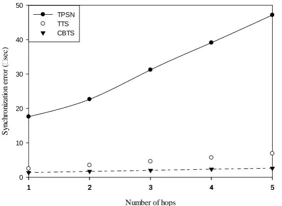
Synchronization error is the difference between the times of a CH with respect to the times of the sink. The synchronization error is added with the increasing number of hops generally. The variation in the synchronization error is studied by fixed number of nodes i.e. 300 nodes, while keeping the sensing field size constant at 300 m. The synchronization error increases with number of hops for CBTS, TTS and TPSN protocols in particular as shown in Figure 10. The values shown in the Figure 10 are the average of 50 simulation results.
Number of hops
1 222 3 444 5
1 2 3 4 5
1 2 3 4 5
S
ync
hr
o
ni
za
tio
n
er
ro
r
(
sec)
0 10 20 30 40 50
[image:17.595.232.519.70.280.2]TPSN TTS CBTS
Figure 10. Variation in propagated synchronization error with number of hops.
uses large number of messages, since several messages bump into each other causing a collision and required to be sent again and leads to error. A large amount of message transmission leads to collisions and further to performance degradation. Synchronization error of TTS is also high because of using a pair of nodes to synchronize the SNs which increase number of messages and adds er-rors at each hop. The performance of cluster based time synchronization (CBTS) is better than other two protocols i.e. 2.6 μs for five hops due to less number of synchronization messages and better clustering approach which reduces the packet collisions and thereby reducing the synchronization error. Simulation results show that our proposed protocol outperforms other protocols in terms of synchronization error. In case of TPSN, the unbalanced clustering technique and the overhead of messages for synchronization are responsible for higher syn-chronization error. CBTS uses EECA clustering technique which required less number of synchronization messages to synchronize the sensor network.
The total time required to synchronize the network is known as convergence time. The variation in the convergence time is studied by fixed number of nodes
Number of hops
1 2 3 4 5
C
o
nv
er
gen
ce
tim
e
(s
)
50 100 150 200 250 300
[image:18.595.232.518.68.277.2]TPSN TTS CBTS
Figure 11. Variation in convergence time with number of hops.
6. Conclusion
The proposed cluster based time synchronization protocol ensures the synchro-nization of the nodes with global time. The proposed CBTS protocol uses the EECA clustering technique proposed in section 2 for clustering the network. Synchronization is performed using top to bottom approach. CHs synchronize with the sink and SNs synchronize with their respective CHs. The proposed technique uses n+2 messages to synchronize the n SNs. Therefore, the pro-posed CBTS is suitable for time synchronization in energy efficiency manner. Simulation results demonstrate the effectiveness of the proposed protocol in terms of message complexity, total energy dissipation per synchronization round, propagated synchronization error, convergence time and synchroniza-tion precision level. The simulasynchroniza-tion results are compared with TPSN and TTS protocols. The proposed CBTS protocol provides better results in comparison with these protocols and can be used in WSNs for less energy consumption and prolonging the network lifetime.
References
[1] Akyldiz, I.F., Su, W., Sankarasubramaniam, Y. and Cayirci, E. (2002) Wireless Sen-sor Networks: A Survey. Computer Networks, 38, 393-422.
[2] Mottola, L. and Picco, G.P. (2011) Programming Wireless Sensor Networks: Fun-damental Concepts and State of the Art. ACM Computing Surveys, 43, Article No.
19. https://doi.org/10.1145/1922649.1922656
[3] Kuorilehto, M., Hännikäinen, M. and Hämäläinen, T.D. (2005) A Survey of Appli-cation Distribution in Wireless Sensor Networks. EURASIP Journal on Wireless Communication and Networking, 2005, Article ID: 859712.
https://doi.org/10.1155/WCN.2005.774
Com-puter Science, Vol. 3824, Springer, Berlin, Heidelberg, 663-672.
https://doi.org/10.1007/11596356_66
[5] Thakur, S., Reddy, M.V., Siddavattam, D. and Paul, A.K. (2012) A Fluorescence Based Assay with Pyranine Labeled Hexa-Histidine Tagged Organophosphorus Hydrolase (OPH) for Determination of Organophosphates. Sensors and Actuators B: Chemical, 163, 153-158.
[6] Thakur, S., et al. (2011) A Flow Injection Immunosensor for the Detection of Atra-zine in Water Samples. Sensors and Transducers Journal, 31, 91-100.
[7] Romer, K., et al. (2002) Middleware Challenges for Wireless Sensor Networks. ACM SINGMOBILE Mobile Computing and Communication Review, 6, 59-61.
https://doi.org/10.1145/643550.643556
[8] Mills, D.L. (1991) Internet Time Synchronization: The Network Time Protocol. IEEE Transactions of Communications, 39, 1482-1493.
https://doi.org/10.1109/26.103043
[9] Mills, D. (1992) Network Time Protocol (Version 3) Specification, Implementation and Analysis. Technical Report, University of Delaware, Delaware.
[10] Mills, D. (1995) Improved Algorithms for Synchronizing Computer Network Clocks. IEEE/ACM Transactions on Networking 3, 245-254.
https://doi.org/10.1109/90.392384
[11] Elson, J., Girod, L. and Estrin, D. (2002) Fine-Grained Network Time Synchroniza-tion Using Reference Broadcasts. 5th Symposium on Operating Systems Design and Implementation, 36, 147-163. https://doi.org/10.1145/1060289.1060304
[12] Elson, J. and Romer, K. (2003) Wireless Sensor Networks: A New Regime for Time Synchronization. ACM SIGCOMM Computer Communication Review, 33, 149- 154.
[13] Romer, K. (2001) Time Synchronization in Ad Hoc Networks. ACM Symposium on Mobile Ad Hoc Networking and Computing, Long Beach, CA, 4-5 October 2001, 173-182. https://doi.org/10.1145/501416.501440
[14] Mock, M., et al. (2000) Continuous Clock Synchronization in Wireless Real-Time Applications. 19th IEEE Symposium on Reliable Distributed Systems, Nurnberg, 16-18 October 2000, 125-133. https://doi.org/10.1109/RELDI.2000.885400
[15] Ganeriwal, S., et al. (2003) Timing-Sync Protocol for Sensor Networks. Internation-al Conference on Embedded Networked Sensor Systems, Los Angeles, CA, 5-7 No-vember 2003, 138-149. https://doi.org/10.1145/958491.958508
[16] Ganeriwal, S., et al. (2003) Network-Wide Time Synchronization in Sensor Net-works. Technical Report, Networked and Embedded Systems Lab, Electronic Engi-neering Department, UCLA.
[17] Maróti, M., et al. (2004) The Flooding Time Synchronization Protocol. 2nd Interna-tional Conference on Embedded Networked Sensor Systems, Baltimore, MD, 3-5 November 2004, 39-49.
[18] Wang, J., et al. (2014) Two-Hop Time Synchronization Protocol for Sensor Net-works. EURASIP Journal on Wireless Communications and Networking,2014, 39-
48. https://doi.org/10.1186/1687-1499-2014-39
[19] Djenouri, D., et al. (2013) Fast Distributed Multi-Hop Relative Time Synchroniza-tion Protocol and Estimators for Wireless Sensor Networks. Ad Hoc Networks, 11, 2329-2344.
[21] Wu, J., et al. (2012) Average Time Synchronization in Wireless Sensor Networks by Pairwise Messages. Computer Communications, 35, 221-233.
[22] PalChaudhuri,, S., et al. (2003) Probabilistic Clock Synchronization Service in Sen-sor Networks. Technical Report TR 03-418, Department of Computer Science, Rice University, Houston.
[23] Li, Q. and Rus, D. (2004) Global Clock Synchronization in Sensor Networks. IEEE Conference on Computer Communications, 1, 564-574.
[24] Ping, S. (2003) Delay Measurement Time Synchronization for Wireless Sensor Networks. Intel Research, IRB-TR-03-013.
[25] Arvind, K. (1994) Probabilistic Clock Synchronization in Distributed Systems. IEEE Transactions on Parallel and Distributed Systems, 5, 474-487.
https://doi.org/10.1109/71.282558
[26] Sichitiu, M.L. and Veerarittiphan, C. (2003) Simple, Accurate Time Synchronization for Wireless Sensor Networks. IEEE Conference on Wireless Communications and Networking, New Orleans, LA, 16-20 March 2003, 1266-1273.
[27] Su, W. and Akyildiz, I. (2005) Time-Diffusion Synchronization Protocols for Sensor Networks. IEEE/ACM Transactions on Networking, 13, 384-397.
https://doi.org/10.1109/TNET.2004.842228
[28] He, L.-M. (2008) Time Synchronization Based on Spanning Tree for Wireless Sen-sor Network. 4th International Conference on Wireless Communications, Net-working and Mobile Computing, Dalian, 12-14 October 2008, 1-4.
[29] Xu, M., Zhao, M. and Li, S. (2005) Lightweight and Energy Efficient Time Synchro-nization for Sensor Network. International Conference on Wireless Communica-tions, Networking and Mobile Computing, 2, 947-950.
[30] Seareesavetrat, S., Pornavalai, C. and Varakulsiripunth, R. (2008) A Light-Weight Fault-Tolerant Time Synchronization for Wireless Sensor Networks. 8th Interna-tional Conference on ITS Telecommunications, Phuket, 24-24 October 2008, 182- 186.
[31] Park, C., et al. (2007) Reference Interpolation Protocol for Time Synchronization in Wireless Sensor Networks. Proceedings of the 4th International Conference on Ubiquitous Intelligence and Computing, Hong Kong, 11-13 July 2007, 684-695. [32] Heinzelman, W.B., et al. (2002) An Application-Specific Protocol Architecture for
Wireless Microsensor Networks. Transactions on Wireless Communications, 1, 660-670. https://doi.org/10.1109/TWC.2002.804190
[33] Chandrasekaran, V. and Shanmugam, A. (2013) An Energy Efficient Multi Hop Hierarchical Routing in Wireless sensor Networks. IOSR Journal of Electronics and Communication Engineering (IOSR-JECE), 5, 61-65.
https://doi.org/10.9790/2834-0546165
[34] Zhao, F., Xu, Y. and Li, R. (2012) Improved LEACH Routing Communication Pro-tocol for a Wireless Sensor Network. International Journal of Distributed Sensor Networks, 1-6.
[35] Manjeshwar, A. and Agrawal, D. (2001) TEEN: A Routing for Enhanced Efficiency in Wireless Sensor Networks. 15th International Parallel and Distributed Processing Symposium (IPDPS), San Francisco, CA, 23-27 April 2000, 2009-2015.
https://doi.org/10.1109/ipdps.2001.925197
[37] Nehra, V. and Sharma, A.K. (2013) PEGASIS-E: Power Efficient Gathering in Sen-sor Information System Extended. Global Journal of Computer Science and Tech-nology, 13, 14-18.
[38] Demirbas, M., et al. (2004) FLOC: A Fast Local Clustering Scheme in Wireless Sen-sor Networks. Workshop on Dependability Issues in Wireless Ad Hoc Network and Sensor Networks (DIWANS).
[39] Zhang, H. and Shen, H. (2009) Balancing Energy Consumption to Maximize Net-work Lifetime in Data-Gathering Sensor NetNet-works. IEEE Transactions on Parallel and Distributed Systems, 20, 1526-1539. https://doi.org/10.1109/TPDS.2008.252
[40] Ferng, H.W., et al. (2012) Energy Efficient Routing Protocol for Wireless Sensor Networks with Static Clustering and Dynamic Structure. Wireless Personal Com-munications, 65, 347-367. https://doi.org/10.1007/s11277-011-0260-4
[41] Wu, X., Chen, G. and Das, S.K. (2008) Avoiding Energy Holes in Wireless Sensor Networks with Non-Uniform Node Distribution. IEEE Transactions on Parallel and Distributed Systems, 19, 710-720. https://doi.org/10.1109/TPDS.2007.70770
[42] Halgamuge, M., et al. (2009) An Estimation of Sensor Energy Consumption. Pro- gress in Electromagnetics Research B, 12, 259-295.
https://doi.org/10.2528/PIERB08122303
Submit or recommend next manuscript to SCIRP and we will provide best service for you:
Accepting pre-submission inquiries through Email, Facebook, LinkedIn, Twitter, etc. A wide selection of journals (inclusive of 9 subjects, more than 200 journals)
Providing 24-hour high-quality service User-friendly online submission system Fair and swift peer-review system
Efficient typesetting and proofreading procedure
Display of the result of downloads and visits, as well as the number of cited articles Maximum dissemination of your research work