http://www.scirp.org/journal/tel ISSN Online: 2162-2086
ISSN Print: 2162-2078
DOI: 10.4236/tel.2017.73033 April 13, 2017
How Can the Error Term Be Correlated with the
Explanatory Variables on the R.H.S. of a Model?
Yunyun Lv
Department of Economics, Kansas State University, Manhattan, KS, USA
Abstract
Since macroeconomic research cannot be replicated, most studies may claim their conclusive research findings solely based on the statistical significance of the estimated coefficients. In this framework, we use a small simulation expe-riment to show that if variables affect the economy through different hori-zons, even though the error term is not correlated with both the explanatory variables on the right-hand side (R.H.S.) of a model and the dependent varia-ble from a traditional view, the estimated coefficients can still be biased. The evidence provided by this paper may explain the refutation and controversy results in the modern research.
Keywords
Cointegration in the Longer Horizons, Simulation
1. Introduction
Published research findings of the relationships among variables are sometimes refuted by subsequent evidence. For instance, Hamilton (1983) [1] shows that oil shocks may be a contributing factor in some of the recessions before 1972. In order to explore the asymmetric effects of oil price on output, Mork (1989) [2] estimates separate coefficients for oil price increase and decrease. Additionally, Hooker (1996) [3] provides evidence that the predictive power of oil shocks on macro variables diminish as the sample is updated. Examples also include that the traditional view in the literature until 2003 espouses that the real price of oil responses to the oil supply shocks more than the oil demand shocks, whereas Ki-lian (2009a) [4] provides evidence that the real price of oil responses to the oil supply shocks less than the oil demand shocks. The sectoral shift hypothesis discusses that it is possible for large oil price changes in either direction to po-tential to hurt output. The instability of the empirical relation between oil price How to cite this paper: Lv, Y.Y. (2017)
How Can the Error Term Be Correlated with the Explanatory Variables on the R.H.S. of a Model? Theoretical Economics Letters, 7, 448-453.
https://doi.org/10.4236/tel.2017.73033
Received: February 9, 2017 Accepted: April 10, 2017 Published: April 13, 2017
Copyright © 2017 by author and Scientific Research Publishing Inc. This work is licensed under the Creative Commons Attribution International License (CC BY 4.0).
449
and output incurs a debate over whether the oil-price-GDP relationship still ex-ists or not. Refutation and controversy are seen in the oil price literature as the data are updated.
Couple studies discuss the increasing concern that the findings claimed by the vast majority of published research are false. Loannidis (2005a [5], 2005b [6]) point out that the poor agreement of subsequent research with initial findings in the most influential medical journals published between 1990 and 2003 and pro-vide some concerns which may cause most published research findings in a scientific field false under reasonable assumptions. Romer (2016) [7] questions the opaque assumptions and the incredible identifications, especially criticizing the “imaginary shocks” in the “post-real” macroeconomic literature. In this pa-per, I use the assumption that variables affect the economy through various time spans to examine how this assumption affects the estimated coefficients of the macroeconomic models and some corollaries thereof through a different pers-pective from the traditional view.
According to the complication of the economy, macroeconomic research cannot be replicated (lack of confirmation from a scientific view). The research discoveries are a consequence of the convenient strategy by simplification. We select couple key variables in the near term by statistical significance, typically for a p-value less than 0.05 and use these variables to claim the conclusive re-search findings for all horizons. However, under my new assumption, variables may be cointegrated through different horizons. For instance, from the Un-biased Forward Rate(UFR) hypothesis which posits the long-run equilibrium between forward and spot exchange rates on the sixth page of Enders (2014) [8], we can assume that forward value of Y can have a long-run equilibrium with
current value of f :
0 1
t s t t s
Y+ =α +α f +Z+
It may exist that both Yt s+ and ft are I(1) and Zt s+ is I(0). If we consider
t
f as the error term, some variable Yt s+ may be correlated with the error term
t
f multiple-step ahead. In other words, under my assumption that variables can
affect the economy through different horizons, even though the estimated error term is not correlated with the explanatory variables on the right-hand side (R.H.S.) of a model in the near term from a conventional perspective, we cannot assert that they must not be correlated through a longer horizon, which may lead to biased estimates of coefficients.
The innovation of this paper is that I show the influence of the estimated coef-ficients when the error term is correlated with the explanatory variables through a long horizon rather than the short horizons by simulation. According to my results, the traditional model may not be sufficient to resolve the real coefficients of relationships among variables when the error term is correlated with variables on the R.H.S. of the model through the long horizons. Hence, the misinterpreta-tion may exist in the literature.
di-450
rections for future research are given in Section 3.
2. Simulation
In this section, I present the details of our evaluations via simulation. The series of simulation results I carried out reflect in part the major aim of the possibility that the long-horizon relationships of the error term and the explanatory va-riables can be ignored by the traditional models.
If the variables on the right-hand side of a model, denoted as xt, are not
cor-related with residuals et, but correlated with the lagged residuals et−1, these variables can take the contributions of factors in the lagged residuals as part of their own coefficients. To verify that, I impose some hypotheses as following:
• Hypothesis 1. The generated exogenous structural innovations are
indepen-dent iindepen-dentically normal distributed (i.i.d.).
• Hypothesis 2. Variables can be cointegrated in the long horizons, which
im-plies that different types of shocks can affect the same variable through dif-ferent horizons, or the same type of shocks may affect difdif-ferent variables through different horizons.
First, I generate three types of shocks u1,t, u2,t, u3,t, while u1,t, u2,t,
( )
3,t 0,1
u ∼N . Then, I assume that u1,t and u2,t−1 affect xt through different
horizons, whereas u2,t−1 affects xt and et−1 through different horizons. To be specific, I assume that variable xt and residuals et take the form of:
1, 2, 1 0.1 0.5
t t t
x = ×u + ×u − (1)
2, 3, 1 0.5 0.1
t t t
e = ×u + ×u − (2)
To exemplify, I begin by drawing 100 normally distributed random values for each type of shocks1. Then, I compute variable
t
x and residuals et by
Equa-tion (1) and EquaEqua-tion (2) and estimate the regressions. After running the above process 10,000 times, I calculate the average estimations of the relationship be-tween xt and et:
1 1 1,
t t t
x =
α β
+ e +ν
(3)2 2 1 2,
t t t
x =
α
+β
e− +ν
(4)where letting βˆ1 and βˆ2 be the Equation (3) & Equation (4) mean estimates
of β1 and β2, respectively. In this paper, I use *** on the right side of p-value to indicate the 0.1% level of significance of the coefficients. According to the re-sults in Table 1, I show that xt and et are not correlated from a standard
view, but xt and et−1 is statistically significantly correlated at a 0.1% level like the possible relationships of variables and the error term in a traditional model. This assumption is reasonable because we may not include all key variables in the model, there may be some vital variables concealed in the residuals which are correlated with both dependent variables and explanatory variables through long time scales.
Then I assume yt in Equation (5):
451
Table 1. Estimations when explanatory variables are correlated with error term one-step ahead.
ˆ
β t-value p-value
1
ˆ
β −0.01 −0.10 0.50
2
ˆ
[image:4.595.204.540.100.153.2]β 0.96 34.48 4.67E−43 ***
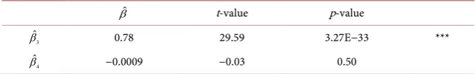
Table 2. Estimations of the model with explanatory variables and error term at the same horizon.
ˆ
β t-value p-value
3
ˆ
β 0.78 29.59 3.27E−33 ***
4
ˆ
β −0.0009 −0.03 0.50
Table 3. Estimations of the model with explanatory variables and error term from differ-ent horizons.
ˆ
β t-value p-value
5
ˆ
β 0.21 2.78 0.05
6
ˆ
β 0.60 8.05 5.45E−08 ***
1 3, 5 0.2 0.6 0.1
t t t t
y = × +x ×e− + ×u − (5)
Our 10,000-time simulation mean results of the following form are in Table 2.
3 3 4 3,
t t t t
y =
α
+β
x +β
e +ν
(6)Comparing the real coefficients I impose in Equation (5) with the estimated results in Table 2, the estimated coefficients of xt and et are biased. The
es-timated coefficient of xt is 0.78, which is almost equal to 0.2 plus 0.6,
indicat-ing that xt takes the effects of et−1 to pretend as its own coefficient. The part which contains the effect of u3,t−1 in et−1 on yt is still concealed in the error
term.
However, our 10,000-time simulation mean results of Equation (7) are near the real coefficients I set in Equation (5):
4 5 6 1 4,
t t t t
y =
α
+β
x +β
e− +ν
(7)In Table 3, when we substitute et by et−1, the estimated coefficients are al-most unbiased. Thus, if there are factors in the error terms which are correlated with the dependent variable and the explanatory variables on the R.H.S. over long horizons, we need to include these factors corresponding to their horizons, respectively. Otherwise, it will be concealed in
ν
3,t in Equation (6) and thees-timated coefficients of variables may be biased. These key variables selected in the near term in the model may take the coefficients of the omitted variables in the error term as their own coefficients.
[image:4.595.206.540.196.248.2]452
3. Conclusions
Under the assumption that the variables may affect the economy through dif-ferent horizons, this paper uses simulations to prove the possibility that the error term can be correlated with both explanatory variables and the dependent va-riables at the same time through longer horizons even though they are not cor-related in the near term through a traditional view. Thus, the estimated coeffi-cients of some traditional models may be biased under my new assumption. Moreover, I argue that it may be misleading to emphasize the statistically signi- ficant findings because some variables in the model may just take the contribu-tions of the omitted variables concealed in the error term. The policy intuition of this paper is that the long-term economic problems cannot be fixed with short- term interventions.
A potential criticism of the approach I implement is that I generate shocks by assuming that these exogenous structural innovations are i.i.d. Likewise, I gen-erate several random shocks from the same distribution. However, the fluctua-tions of the real economic time series may not be from random shocks, but from shocks controlled by the information over different horizons. Additionally, these shocks may be correlated with each other through different horizons. Since my primary focus is to document the change in the estimated coefficients when shocks affect the economy through different horizons, the property of shocks may not affect my results that much. I do not think that this limitation is overly problematic. Nonetheless, the real economic activities are much more complex than my oversimplified simulation experiment. I am only interested in providing the possibility of how my assumption may affect the estimated coefficients of macroeconomic models, as opposed to claiming that my assumption reflects the mere fact of the economy in this paper.
Some concerns for future research are as followings:
First, the biased coefficients may be useful for forecasting since the relation-ships among variables in the economy were relatively stable. If the economy is not in a recession, the stable relationships among variables may lead to a good forecasting performance even without cause relationships. Nevertheless, we need to be as careful as possible to use the estimated coefficients of a linear model like OLS to explain the relationship among variables because part of the coefficients may be from the outside variables in the error term.
Second, some variables which play small roles when adopting a short-run perspective may affect the economy strongly in the long-time horizon, so we may need to select macroeconomic variables specific to the horizon.
453
Overall, if we change the assumption, the conclusions inferred from the biased coefficients of traditional models are by no means settled issues. It remains pos- sible for a skeptic to maintain some dominant views of existing studies which are derived from the biased coefficients. These concerns are beyond the scope of this paper and needed to be further studied.
References
[1] Hamilton, J.D. (1983) Oil and the Macroeconomy Since World War II. The Journal
of Political Economy, 91, 228-248. https://doi.org/10.1086/261140
[2] Mork, K.A. (1989) Oil and the Macroeconomy When Prices Go up and down: An
Extension of Hamilton’s Results. Journal of Political Economy, 97, 740-744.
https://doi.org/10.1086/261625
[3] Hooker, M.A. (1996) What Happened to the Oil Price-Macroeconomy
Relation-ship? Journal of Monetary Economics, 38, 195-213.
[4] Kilian, L. (2009) Not All Oil Price Shocks Are Alike: Disentangling Demand and
Supply Shocks in the Crude Oil Market. American Economic Review, 99, 1053-
1069. https://doi.org/10.1257/aer.99.3.1053
[5] Ioannidis, J.P. (2005) Contradicted and Initially Stronger Effects in Highly Cited
Clinical Research. JAMA, 294, 218-228. https://doi.org/10.1001/jama.294.2.218
[6] Ioannidis, J.P.A. (2005) Why Most Published Research Findings Are False. PLoS
Medicine, 2, e124.
https://doi.org/10.1371/journal.pmed.0020124
[7] Romer, P. (2016) The Trouble with Macroeconomics. The American Economist,
forthcoming.
[8] Enders, W. (2014) Applied Econometric Time Series. 4th Edition. John Wiley, New
York.
Submit or recommend next manuscript to SCIRP and we will provide best service for you:
Accepting pre-submission inquiries through Email, Facebook, LinkedIn, Twitter, etc. A wide selection of journals (inclusive of 9 subjects, more than 200 journals)
Providing 24-hour high-quality service User-friendly online submission system Fair and swift peer-review system
Efficient typesetting and proofreading procedure
Display of the result of downloads and visits, as well as the number of cited articles Maximum dissemination of your research work
Submit your manuscript at: http://papersubmission.scirp.org/