SBAM: An algorithm for pair matching

Munich Personal RePEc Archive

SBAM: An algorithm for pair matching

Stephensen, Peter and Markeprand, Tobias

DREAM

31 October 2013

Online at

https://mpra.ub.uni-muenchen.de/59580/

SBAM: An Algorithm for Pair Matching

∗

Peter Stephensen & Tobias Markeprand, DREAM

October 31, 2013

Abstract

This paper introduces a new algorithm for pair matching. The method is

called SBAM (Sparse Biproportionate Adjustment Matching) and can be

char-acterized as either cross-entropy minimizing ormatrix balancing. This implies

that we use information efficiently according to the historic observations on

pair matching. The advantage of the method is its efficient use of information

and its reduced computational requirements. We compare the resulting

match-ing pattern with the harmonic and ChooSiow matchmatch-ing functions and find that

in important cases the SBAM and ChooSiow method change the couples

pat-tern in the same way. We also compare the computational requirements of the

SBAM with alternative methods used in microsimulation models. The method

is demonstrated in the context of a new Danish microsimulation model that

has been used for forecasting the housing demand.

∗_{Financial support from the Knowledge Centre for Housing Economics, Realdania is gratefully}

acknowl-edged.

1 Introduction

Dynamic microsimulation finds increasing use in demographic and socioeconomic

fore-casting. A big advantage of the microsimulation approach is that it makes it possible

to analyze family structure. In traditional population projections the goal is usually to

forecast the population by age, gender and a few other characteristics (such as origin

and/or geographical region) while the family structure is ignored. Thus children and their

parents are unrelated in the model, as is the typical prerequest for parenthood:

match-ing of couples. Introducmatch-ing family structure into this approach is problematic, mainly

because the size of the model increases tremendously when forecasting the population by

family/household characteristics. These characteristics can alternatively be analyzed in a

microsimulation model without loosing control over the size of the model.

Modelling the family structure requires some extra features compared to the traditional

approach. To get the family composition right, at least two things are necessesary: Parity1

must included in the fertility determination, and pair matching must be modelled. This

paper deals with the latter subject and introduces a new algorithm for pair matching.

A fundamental issue in the pair matching methodology and the event of coupeling

compared with most traditional demographic events modelled in microsimulations is the

coordination nature. While mortality, emigration, fertility etc. are person or household

specific events, coupeling needs the coincidence of events between two independent

house-holds/persons.

Usually two distinct methodologies are mentioned when it comes to matching: the stable

marriage approach (previously used in the CORSIM and DYNACANE models) and the

stochastic approach (used in the DYNASIM model). The method decribed in this paper

cannot be categorized as either, which use a method known from other economic and/or

statistical problems, known as thebalancing matrix method.

In the stable marriage approach the matching is determined by a behavior derived from

(rational) preferences. A matching of a pool of individuals is stable in this context if you

cannot form a new pair which improves both individuals well-being. Theoretically, it was

shown by Gale & Shapley (1962) that such an stable matching always exists and they

fur-thermore provides an algoritme to find such a stable matching. The advantage is obviously

that if the preferences are known you obtain more correct observable matchings which are

more stable. Further, changes in matching patterns are explainable by well-known

con-cepts as demand and supply. The method has at least two drawbacks in the application

to simulation: first of all, the correctness is conditional upon the estimation of preferences

and that the actual matching occurs as if the algorithme determines the matching.

Sec-ond, the matching algorithme is very computational demanding since one needs to match

directly each pair, one by one. Whereas in genuine stable matching algorithms where

each person state his/her ordering of mate, the matching in more applied approaches is

based upon a “compatibility index”, reflecting the likelihood that they are matched. The

mechanism then is as follows: pair any potential couple and estimate the compatibility

index and match the pair with the highest index value. Exclude these persons from the

pool and match the remaining pairs with higest index value. Repeat until the pool of is

empty.

In the stochastic approach one estimates the probability of a match by the difference in

characteristics, like e.g. age and education. The matching procedure then proceed by

pair-ing uspair-ing the Monte Carlo method. The method is generally very coarse in its predictions

of matching pairs and equally computational demanding a like the stable approach.

The method that we introduce, called SBAM (Sparse Biproportionate Adjustment

Matching), can be characterized as either cross-entropy minimizing or matrix balancing

(defined below). The SBAM method is based on historical observations of pair mathings

from one or more years, distributed on a set of types (age, gender, education, geographical

region ect.). In a forecasted year, it is assumed that a matching pool of individuals has

data, the matching problem is easy to solve: We simply distribute the pairs as in the

historical data. If this is not the case (which it typically is not), the pairs must be

dis-tributed in a new way. But how should the distribution be adjusted? and what principles

should apply to these adjustments? One principle could be to distribute the pairs such

that the distribution deviates as little as possible from the historical distribution. This

can be interpreted as a so-called matrix balancing problem (Schneider & Zenios, 1990):

Change the original data (defined as a matrix) such that the row and column sums are

given by predefined values. A number of solutions exist to this kind of problem. One such

solution is called biproportionate adjustment (or RAS adjustment). This method has at

least two advantageous properties: It is relatively easy to implement, and it has a nice

interpretation. Further, the matrix entries preserve the signs after the adjustment. Using

biproportionate adjustment, the outcome can be interpreted as the result of a so-called

cross-entropy minimization problem (McDougall, 1999). In other words, the adjusted

matching changes the distribution of pairs relative to the original distribution, so that

the information loss is as small as possible. The information loss is defined by Shannon’s

Information Theory (Shannon, 1948).

Section 2 decribes the methodology of the matching method. Section 3 analyze the

matching function induced by the RAS method by comparing the properties to two other

matching functions: the harmonic and Choo-Siow matching functions. The comparison is

carried out by considering the changes in the distributions when the population

character-istics change. Section 4 compare the calculation complexity of the SBAM method to other

pratical matching processes used in dynamic microsimulation models. Section 5 shows

an application of SBAM in a new Danish microsimulation model in which we compare

historical observed matching distributions with the SBAM model’s predictions. We also

explain why the methodology of the Choo-Siow matching function is not suitable for the

2 Methodology

There are assumed to be N individuals to be matched into pairs2. The individuals are

divided intoT types:

N =

T

X

j=1

Nj

A type could for example be defined on the basis of gender, age, origin and education.

The numberT can therefore be expected to be rather large3.

The aim is to find real numbersxi,j (i= 1, ..., T, j = 1, ..., T) such that

T

X

j=1

xij =Ni, i= 1, ..., T (1)

and

xij =xji, i, j= 1, ..., T (2)

The matching is defined by (1). The variable xij indicates the number of individuals of

typeithat are paired with an individual of typej. If an individual of typeiis paired with

a person of typej, then the opposite is also the case: An individual of type j is paired

with a person of typei. This gives rise to the symmetry assumption (2).

2.1 Data

The algorithm is based on data from actual matchings. Letx0_ijbe the number of individuals

of typei that according to data is matched with an individual of type j. As mentioned

above, the data setx0_ij is symmetric. This is ensured in the following way: When a pair

2_{N is assumed to be an even number.}

3_{As an example, assume the types are defined on the basis of 2 genders, 50 ages (15-65), 5 education}

of type (i, j) is added to data, it is done by following the procedure:

x0_ij =: x0_ij + 1

x0_ji =: x0_ji+ 1

where =: is an algorithmic equal sign4. In the data set, individuals are distributed on T

types:

N_t0 =

T

X

i=1

x0_it=

T

X

j=1

x0_tj (3)

and the total number of individuals is given by

N0 =

T

X

j=1

N_j0

It is advantageous to describe the problem in matrix notation. The data set x0_ij can be

described as aT_×T matrix,X0.Define the vector

~

N0 = N₁0, ..., N_T0

According to (3), both the row and column sums ofX0 should be given byN~0.

2.2 Biproportionate Adjustment

We are going to matchN individuals, distributed on types according toN~ = (N₁, ..., NT).

We wish to find a T_×T dimensional symmetric matrix X such that its row and column sums add to N~. This should be done so that X deviates as little as possible from the

original data X0. In other words, we would like our matching X to reflect as much as

possible of the matching information in the original (real world) matching X0. This can

be interpreted as a classical matrix balancing problem: Given a rectangular matrix A,

determine a matrix X that is close to A and satisfies a given set of linear restrictions on

its entities (Schneider & Zenios, 1990).

Algorithms for matrix balancing can be separated into two broad classes: scaling

algo-rithms and optimization algoalgo-rithms. Scaling algoalgo-rithms multiply the rows and columns of

the original matrix by positive constants until the matrix is balanced. Optimization

algo-rithms minimize a penalty function that measures the deviation of a candidate balanced

matrix from the original matrix. The balance conditions are constraints in the

optimiza-tion model, so that the optimal soluoptimiza-tion is the balanced matrix closest to the original

matrix.

We are going to use the scaling approach here. According to the biproportionate

adjust-ment model (also called RAS adjustadjust-ment), the balancing problem can be solved in the

following iterative way: Start with the original matrix. Scale the rows such that the row

sums are correct. Then scale the columns such that the column sums are correct. Repeat

these two operations until a new stable matrix has emerged.

When using the optimization algorithms, it is obvious that the new matrix deviates

as little as possible from the original matrix (that is part of the definition of the

prob-lem). This is less obvious when it comes to the scaling algorithms. However, it has been

demonstrated that the biproportionate model is an entropy-theoretic model (see e.g.

Mc-Dougall, 1999 or Bregman, 1967). The new matrix can be characterized as the solution to

a cross-entropy minimization model. Entropy should here be understood in an information

theoretical context (Shannon, 1948). By using the biproportionate model we are actually

minimizing the loss of information when changing from the type distributionN~0 toN~.

The balancing condition in this particular problem is

T

X

i=1

T

X

j=1

xij =Ni

for everyi, j = 1, . . . , T. Note that this impose a symmetry in the balancing conditions

whenever the row and column indice is the same.

The procedure for the RAS algorithm is as follows: for anyk let

1. fori= 1, . . . , mlet ρk_i = PNi

jxkij

and let yk_ij =ρk_ixk_ij for all i= 1, . . . , m;j= 1, . . . , n

2. forj= 1, . . . , nletσk_j = PNj

iykij

and letxk_ij+1=σk_jy_ijk for alli= 1, . . . , m;j = 1, . . . , n

Letting X0 = X₀ the RAS-solution is the limit XRAS _{= lim}

k→∞Xk. It is easy to see that we can write the solution in the terms of a matrix product: lettingR be them_×m

diagonal matrix with elements

rii=

∞

Y

k=1

ρk_i

andS then_×ndiagonal matrix with elements

sjj =

∞

Y

k=1

σk_j

Then we can write the solution to the RAS algorithm asXRAS=RX0S.

An important property of the RAS algorithm, in our context, is that it preserves

sym-metry of the initial distribution when the balancing conditions are symmetric. Symsym-metry

implies that for eachk we have thatxk_ij+1 =xk_ji+1 whenever xk

ij =xkji. But we have that

xk_ij+1 = σ_jky_ijk = _PNj

iykij

yk_ij = _PNj

iρkixkij

ρk_ixk_ij = _P Nj

i Ni

P

jxkij

xk ij

Ni

P

jxkij

xk_ij

= Ni

P

j Nj

P

jxkij

xk ji

Nj

P

ixkij

xk_ji =xk_ji+1

the solution considerably reduce the computational requirements by reducing the

compu-tations by 50%. However, this may still be a considerable computational accomplishment

depending on the number of types and the convergence of the iterative procedure.

As we have mentioned, the solution of the RAS method is equivalent to the solution

of a well-defined minimization problem. It has been shown that the RAS solution is the

solution to the problem of minimizing of the cross entropy

min (ξij)_i,j

X

i,j

ξijlog

ξij

ξ_ij0

subject to the balancing condition whereξij = xij_Ni and ξij0 = x0

ij N0

i

.

The RAS algorithm has a well-known graph structure associated with it, which is

valu-able for understanding the mathematical structure. A graph is a pair (V, E) where V is

the set of vertices and E the set of arces a subset of V _×V. Given two vertices iand j

we say that they are connected in the graph (V, E) if (i, j) _∈ E or (j, i) _∈ E, that is if there exists an arc connecting the two vertices. A graph isbiparitite if there exists adjoint

subsets V1, V2 ⊂ V that covers Vsuch that for every i ∈ V1 there exists an j ∈ V2 and (i, j)_∈E. We can now define the transportation graph for the RAS algorithm: GivenX0

we denote byV1 the set of rows and V2 the set of columns and we let the transportation

graph be the biparitite graph (V, E) given by

V =_{1, . . . , m_{} ∪}

1′, . . . , n′ =V1∪V2

and

E=

i, j′

∈V_1×V_2|x0_ij′ >0

whereV2 ={1′, . . . , n′} is just a relabelling of{1, . . . , n}to distinguish elements from the two setsV1 and V2. Hencefourth, we will refer to arces as (i, j) instead of (i, j′) when no

absence of a zero row (column). The matrixX0 can then be identified by the positive map

x0 :E_−→R+. The RAS algorithm then cycles through the transportation graph scaling the mapX0 on the transportation graph such that the limit satisfies

X

{j|(i,j)∈E}

xij =Ni

for everyi_∈V1 and

X

{i|(i,j)∈E}

xij =Nj

for everyj_∈V2. It is important to note that there are computational differences between the matrix algorithm and the graph algorithm, since the former requires computations for

allT2 entries, while the latter only refer to the subset of these elements in which there are

a strictly positive entry.

2.3 Sparse algorithm

As mentioned above, the number of typesT can and will in applications often be very large.

Therefore, a T_×T matrix can easily become so large that it gives rise to computational problems. As there at the same time often will be many zeros in the X0 matrix, it will

have obvious advantages to introduce a sparse matrix method in which operations on

zero-elements are ignored. The method is implemented in C# and is based on so-calledlinked

lists5. A T _×T matrix can be represented by a SBAMMatrix. A SBAMMatrix is a C#

object that essentially contains 2T linked lists: T linked lists for the rows and T linked

lists for the columns. Each element in the linked list contains a pointer to data and a

reference to the next element in the list. In this way, data is actually represented twice: as

rows and as columns. The motivation for this redundancy is that it makes biproportionate

5_{A linked list is a data structure consisting of a group of nodes that together represent a sequence. Each}

scaling much easier. The SBAMMatrix actually implements the graph structure of the

RAS algorithm, as described above.

3 Matching functions

A well-known characterization of reduced form matching models is through the use of

matching functions. In terms of the model in this paper, a matching function is a map

µij(N) ∈R which gives the number of matchings between type iand type j individuals

given a population N. This section provides a comparison of the resulting steady state

matching pattern of the SBAM method with two other important methods: the harmonic

mean method and the Choo-Siow method.

Traditionally, the definition has been termed a bit differently which is contained in our

formulation. To arrive at the traditional formulation one can separat the setN =M_∪F

whereM is the set of males to be matched andF is the set of females to be matched. Then

µij(M, F) is the number of males of type i to be married to females of type jdependent

on the number of all males and females to be matched. In the present model we allow

persons of the same gender to form relationships, which the traditional formulation does

not allow.

The matching function usually satisfies some properties (beyond the balancing

condi-tions):

• Zero spillover: letting Ni be the number of typei, thenµij(N) =µij(Ni, Nj)

• Homogenity of one: for any scalar λ >0 we have that µij(λN) =λµij(N)

The zero spillover property implies that the matching of pairs of given types only depend

on the number of each type. This implies that nosubstitutioneffect is possible: “if I cannot

An example of this is Harmonic Mean matching function (see Schoen (1988))

µHM_ij (M, F) =αij

mifj

mi+fj

=µHM_ij (mi, fj)

whereαij >0,Piαij ≤1 and Pjαij ≤1. Note that the sum of each type

X

j

µij(M, F) =mi

X

j

αijfj

mi+fj ≤

mi

X

j

fj

mi+fj ≤

mi

such that the total number of matches assigned to typei-males is less than the total number

of typei-males. And likewise forj-type females. Thus, the proportions of married men of

typeiis then given by

ρi(M, F) =

P

jµij(M, F)

mi

=X

j

αij

fj

mi+fj

while the proportion of married females ηj(M, F) is defined likewise. The remainning

males/females is not matched, and is given by

µi0= (1−ρi(M, F))mi=

 

X

j

mi+ (1−αij)fj

mi+fj

 mi

and

µ0j = (1−ηj(M, F))fj =

X

i

fj+ (1−αij)mi

fj+mi

!

fj

which we note are all strictly positive and less than one. We note that these rates are

all dependent on, and thus changes whenever, the number of male/females changes. The

change in the individual matching parameters are

      ∂µij ∂mi ∂ρi ∂mi ∂ηi ∂mi ∂µij ∂fj ∂ρi ∂fj ∂ηi ∂fj       =       αij _f j mi+fj

2

αij

mi mi+fj

2

−P

jαij fj

(mi+fj)2 αij

mi

(mi+fj)2

αij_(mifj_+fj)2 − P

where we see that there is a crowding out effect: as there becomes more of one type

of males, this implies that the proportion of married males of this type decreases. An

important proporty of the harmonic mean matching function is that it is homogenous of

degree one, that is the ratios of marriage propensities is affected by a scaling of the number

of men and females:

µij(λM, λF) =µij(λmi, λfj) =λµij(mi, fj)

for anyλ >0. The interpretation of this proporty is that the searching/matching process is

made easier by the presence of a larger set of supply of possible matches. Note, however,

that the proportion of married men/female of a given type is not affected by a

equi-proportional increase in the men and female of the type, i.e.

ρi(λM, λF) =ρi(M, F)

A second example is the Pollard/Hohn matching function given by

µij =

aimibjfj

1 2

P

k(hkjakmk+hikbjfj)

whereai,bj andhij are parameters/weights to be estimated,mi is the number of men of

typeiand fj is the number of females of type j.

A third example is the Choo/Siow matching function given by

µij =πij√µi0µ0j

where πij is a parameter to be estimated which represents the sum of gross benefits of

typeiand j of a matching of the two types in excess of being single,µi0 is the number of

of type j, both derived residually. Choo & Siow (1993) derives the matching function

from a transferable utility model of matching model. Since, by definition, the number of

married men and the number of unmarried men exhaust the males of a given typei

µi0+

J

X

j=1

µij =mi

and likewise for females

µ₀j+ I

X

i=1

µij =fj

we have that a solution for(µi0)i,(µ0j)j

must satisfy

mi−µi0 =

J

X

j=1

πij√µi0µ0j

and

fj−µ0j = I

X

i=1

πij√µi0µ0j

which is basically a quadratic form.6 _{Changes in the parameters ((m}

i),(fj),Q) can

determine the changes in the unemployment rates (µi0, µj0)ij which can then be used for

calculating the change in the distribution of marriages.

It is easy to see that our derived matching function violates the zero-spillover property

but satisfies the homogenity of one property. All the above examples also satisfies the

homogenity property, which is a property that implies that the number of pairs matched

does change with a general increase in the population, and thus that the population density

does not affect the ability of matching. The SBAM contains a very general spillover effect,

in that, not only does the matching of say a type i to a type j depend on any other

match of typei with any other type j′, but also on the matching of type i′ ₆=iwith any

6_{Make the transformation ˜µ}

ij=µ2ijthen the equation for males of typeibecomesmi−µ˜2i0= P

jπijµ˜i0µ˜0j

other typej′. A second important aspect in which our matching function differ from the

mentioned, is that the proportion of matched pairsρandηare independent of the number

of males/females of the different types.

3.1 Comparing matching functions

To see the potential effect of considering the joint distribution when marginal distributions

pertubates, consider the initial distribution

               

0 0 0 10 3 1

0 0 0 5 10 5

0 0 0 1 3 10

10 5 1 0 0 0

3 10 3 0 0 0

1 5 10 0 0 0

               

where the first three rows (columns) are men (with 3 types) and the last three rows

(columns) are female (with 3 types). Thus the initial row/column sums areN0 = (14,20,14,16,16,16).

The population vector is initially given by L0 = (20,25,17,20,20,20) such that the

pro-portion of married of each type is (ρ, η) = (0.7,0.8,0.82,0.8,0.8,0.8). Assume that 5 males

of the first type is added to the total population, such thatL= (25,25,17,20,20,20), how

does this change the matching distribution? The unmarried proportions are changed to

ρHM, ηHM= ((0.62,0.8,0.82),(0.86,0.82,0.81))

for the harmonic mean matching function, and

which implies that the number of couples increase by 1.3 in the HM-case and 1.6 in the

CS-case. The resulting pair-matching of the two matching functions are

µHM =

               

0 0 0 11.1 3.3 1.1

0 0 0 5 10 5

0 0 0 1 3 10

11.1 5 1 0 0 0

3.3 10 3 0 0 0

1.1 5 10 0 0 0

               

, µCS =

               

0 0 0 11.1 3.5 1.2

0 0 0 4.7 9.9 5

0 0 0 0.9 2.9 10

11.1 4.7 0.9 0 0 0

3.5 9.9 2.9 0 0 0

1.2 5 10 0 0 0

               

from which we see that the main difference between the two types of matching functions

is the cross-type effect which is zero in the HM-case and non-zero in the CS-case. The

interpretation is that a greater number of males increases the competition on the

male-side, which increases the demand for females and the supply of males. Like any traditional

economic mechanism would predict this would lower the relative price of males and

sym-metrically increase the relative price of females. This would force males to increase their

utility-transfer to females and thus more females would be attracted to move from being

single to engage in marriage, while spur relatively more males to be singles.

Consider now the resulting change in a SBAM procedure. Unfortunately, the SBAM

and the CooSiow (and also the Harmonic Mean) matching procedures are in there most

basic form in some sense incomparable. To see why, consider an increase in the male

population of, say, type 1. For a given number of females, of each female-type, the number

of couples could not increase if the number of females are not increased as well. In the

CS- matching this is accomblished by an increase in the benefit of each female and thus

new females are attracted to the market for matches. However, in the SBAM the number

of females is unchanged, since the proportion of unmarried is unchanged. However, the

procedure requires that any married individual as predicted by the fixed marriage

same-sex matchings. Recall, however, that matchings do not necessarily imply a sexual

relationship, but instead implies a common household. So in order to make the two (three)

models comparable we now extend the harmonic mean and Choo-Siow models to allow

for the possibility of same-sex matchings. Further, to be able to compare the HM- and

CS-functions with the SBAM we also need to assume that in each period all couples are

dissolved and the entire population must be rematched. The need for this assumption is

discussed in section 5 and has to do with stock and flow models.

The extension is straight forward and present no mentionable technical difficulties. The

observed matchings are now altered to be

               

1 0 0 10 2 1

0 1 0 4 10 5

0 0 1 1 2 10

10 4 1 0 0 0

2 10 2 0 0 0

1 5 10 0 0 0

               

such that the marginal propensities of ’marriage’ are unchanged, given by

(ρ, η) = ((0.70,0.80,0.82),(0.75,0.70,0.80))

. The effect of an increase in the number of type 1-males by 5 individuals on the propensity

to marriage is then

ρHM_{, η}HM

ρCS_{, η}CS

ρSBAM, ηSBAM

=

((0.63,0.80,0.82),(0.81,0.71,0.81))

((0.65,0.79,0.82),(0.79,0.72,0.81))

((0.70,0.80,0.82),(0.75,0.70,0.80))

the distributions are

µHM =

               

1.3 0 0 11.1 2.2 1.1

0 1.0 0 4 10 5

0 0 1.0 1 2 10

11.1 4 1 0 0 0

2.2 10 2 0 0 0

1.1 5 10 0 0 0

               

, µCS =

               

1.5 0 0 11.1 2.4 1.2

0 1.0 0 3.7 10.0 5

0 0 1.0 0.9 2.0 10

11.1 3.7 0.9 0 0 0

2.4 10.0 2.0 0 0 0

1.2 5 10 0 0 0

                ,

µSBAM =

               

3.0 0 0 10.8 2.5 1.3

0 1.8 0 3.4 9.7 5.1

0 0 1.7 0.8 1.8 9.7

10.8 4.7 0.9 0 0 0

2.5 9.7 1.8 0 0 0

1.3 5.1 9.7 0 0 0

               

To give a more proportional feeling of the magitudes of the change, we can compute the

percentage change in the distributions of matchings

µHM =

               

0.25 0 0 0.11 0.11 0.11

0 0 0 0 0 0

0 0 0 0 0 0

0.11 0 0 0 0 0

0.11 0 0 0 0 0

0.11 0 0 0 0 0

               

, µCS=

               

0.47 0 0 0.11 0.18 0.19

0 0.05 0 ₋0.06 0.00 0.00 0 0 0.03 ₋0.07 ₋0.01 0.00 0.11 ₋0.06 ₋0.07 0 0 0 0.18 0.00 ₋0.01 0 0 0 0.19 0.00 0.00 0 0 0

µSBAM =                

1.97 0 0 0.08 0.23 0.28

0 0.85 0 ₋0.15 ₋0.03 0.01 0 0 0.68 ₋0.19 ₋0.08 ₋0.03 0.08 ₋0.15 ₋0.19 0 0 0 0.23 ₋0.03 ₋0.08 0 0 0 0.28 0.01 ₋0.03 0 0 0

               

We note that in general the SBAM result in much greater sensitivities towards the number

and distribution of partnerships than the other matching functions. This greater sensitivity

mainly comes from the constantness of the proportions of marriage, which translate into

a considerable increase in the same-sex ’marriages’.

Consider next a simultanous increase of five persons of type 1- males and -females. The

percentage change in the distributions are

µHM =

               

0.25 0 0 0.25 0.11 0.11

0 0 0 0.13 0 0

0 0 0 0.10 0 0

0.25 0.13 0.10 0 0 0

0.11 0 0 0 0 0

0.11 0 0 0 0 0

               

, µCS=

               

0.26 0 0 0.28 0.12 0.12

0 ₋0.04 0 0.12 ₋0.02 ₋0.02 0 0 ₋0.01 0.14 ₋0.01 ₋0.01 0.28 0.12 0.14 0 0 0

0.12 ₋0.02 ₋0.01 0 0 0 0.12 ₋0.02 ₋0.01 0 0 0

                ,

µSBAM =

               

0.47 0 0 0.30 0.05 0.12

0 0.15 0 0.15 ₋0.07 ₋0.01 0 0 0.15 0.15 ₋0.07 ₋0.01 0.30 0.15 0.15 0 0 0

0.05 ₋0.07 ₋0.07 0 0 0 0.12 ₋0.01 ₋0.01 0 0 0

               

the same-sex matchings are substitutes (when the supply of type 1-population increase,

their matching-price/value decrease which in the case of CS implies that the demand for

same-sex matchings decrease, which is the definition of (gross) substitutes) the same-sex

matchings are complements.

To consider the effect of a symmetric initial condition, in which there are female, as well

as male, same-sex relationships, we consider an alternative initial observation given by

               

1 0 0 9 2 1

0 1 0 4 9 5

0 0 1 1 2 9

9 4 1 1 0 0

2 9 2 0 1 0

1 5 9 0 0 1

               

in which case we obtain per centage change with only type 1-males increase, the marriage

rate of the different changes as (HM)

(ρ, η) = ((0.65,0.76,0.76),(0.75,0.7,0.8))_⇒(ρ, η)HM = ((0.58,0.76,0.76),(0.80,0.71,0.81))

and for CS

(ρ, η)CS= ((0.6,0.75,0.76),(0.78,0.71,0.81))

in which only male relationships where present, and the distributions change by

µHM =

               

0.25 0 0 0.11 0.11 0.11

0 0 0 0 0 0

0 0 0 0 0 0

0.11 0 0 0 0 0

0.11 0 0 0 0 0

0.11 0 0 0 0 0

               

, µCS=

               

0.43 0 0 0.12 0.17 0.18

0 0.03 0 ₋0.05 0.00 0.00 0 0 0.02 ₋0.06 ₋0.01 0.00 0.12 ₋0.05 ₋0.06 ₋0.13 0 0 0.17 0.00 ₋0.01 0 ₋0.04 0 0.18 0.00 0.00 0 0 ₋0.03

                ,

µSBAM =

               

1.42 0 0 0.12 0.24 0.29

0 0.52 0 ₋0.11 ₋0.02 0.02 0 0 0.41 ₋0.14 ₋0.05 ₋0.01 0.12 ₋0.11 ₋0.14 ₋0.48 0 0 0.24 ₋0.02 ₋0.05 0 ₋0.37 0 0.29 0.02 ₋0.01 0 0 ₋0.31

               

and when we consider both male and female type-1 increase the marriage propensities are

(ρ, η)HM = ((0.63,0.78,0.77),(0.72,0.71,0.81))

and

and the distributions becomes

µHM =

               

0.25 0 0 0.11 0.11 0.11

0 0 0 0.13 0 0

0 0 0 0.10 0 0

0.25 0.13 0.10 0.25 0 0

0.11 0 0 0 0 0

0.11 0 0 0 0 0

               

, µCS=

               

0.26 0 0 0.28 0.12 0.12

0 ₋0.03 0 0.12 ₋0.02 ₋0.02 0 0 ₋0.01 0.13 ₋0.01 ₋0.01 0.28 0.12 0.13 0.30 0 0

0.12 ₋0.02 ₋0.01 0 ₋0.01 0 0.12 ₋0.02 ₋0.01 0 0 0.00

                ,

µSBAM =

               

0.25 0 0 0.31 0.12 0.14

0 ₋0.07 0 0.12 ₋0.03 ₋0.02 0 0 ₋0.04 0.14 ₋0.02 ₋0.01 0.31 0.12 0.14 0.36 0 0

0.12 ₋0.03 ₋0.02 0 0.00 0 0.14 ₋0.02 ₋0.01 0 0 0.03

               

Again, it it extremely noteworthy that the changes in the distributions of ChooSiow and

the SBAM are very similar, and in this case in which both same-sex relations are considered

actually the magnitudes of the changes are almost the same. These results suggests that

we can use the SBAM-approach in the microsimulation but use the interpretations from

the CS-approach when interpreting the actual simulation results. A further notice is that

the change in distribution with a proportional increase in the male and female of a given

type is highest in the diagonal and same-sex of the increased male-female types. Compared

to the asymmetric increase in which the sensitivities of the distributions of SBAM and CS

are more dislike, however, they agree on the trend that the same-sex match of the increase

type have uniformly the greatest sensitivity.

Like the rate of matchings is independent of the population size and distribution in

harmonic mean and ChooSiow the dissolvement rate changes as the size and distribution

of the population changes.

4 Alternative microsimulation matching procedures

We shall here consider the matching process used in the DYNASIM and CORSIM/DYNACAN.

Both methods takes the propensity to marriage as exogenous: the probability to be

mar-riaged given age, gender, education and labour market status within a given period is

independent of the population distribution.

4.1 DYNASIM-like procedures

In the DYNASIM model, the matching pool is then randomly queued of males and females

in separate lines. Take the first male in the queue, call himi, and start in the female line

by picking the first female, call herj, and assign the probability7

Pr_{xij = 1}= exp

−1₂

q

(ai−aj)2+ (ei−ej)2

of these two individuals to form a pair. If they are not matched the male i is trialed a

match with the next female in the queue using the same procedure as above. If the male

is not matched within 10 trials he is matched with the femail with the highest probability

estimated in the trials. Any asymmtry in the number of male and females are handled by

leaving the unmatched single and letting them indure the risk of marriage next year.

To calculate the average number of computations necessary to complete the matching

proces, with only age as the determining parameter, consider the probability distribution

of a 30-year old male, given that we match this male with a randomly chosen female the

probability that they will be matched is the expectation of the distribution, e.g. ca. 3 per

7_{This is based upon the presentation of Perese (2002), but it seems an flawed presentation because there}

cent, in the next step the conditional expectation is the same, given that the population is

large, such that the probability of not having found a mate withinn_≤10 trials is (1₋3%)n and thus a probability that having found a mate after exactly n trials is 1₋(1₋3%)n and the probability that exactly at thenround is

Pr_{τ _≤n₋1_{} −}Pr_{τ _≤n_}

which implies that there is about 70% chance that we need more than 10 trials to match

the inidividual. Thus the expected number of trials are 8.5 trials per individual. Assume

that there areN = min_{F, M_} individuals are to be matched, then the expected number of calculations are 8.5_∗N calculations. The resulting distribution of matchings is a very complex and intransparent distribution which would generally depend upon the number

of trials.

4.2 CORSIM-like procedures

In the CORSIM/DYNACAN model, the matching pool is as follows: let there beN persons

in the matching pool, then the procedure estimates N2 = N _∗N probabilities using a estimate as follows: let there beN0individuals observed and variables

n

(yij, xij)_i,j=1,...,N0

o

in whichyij is a dummy equal to one if individualiandjare married, andxij are variables

such as the difference in age, difference in age squared, difference in years of education,

labourforce status, difference in earnings etc. including interaction terms and then estimate

the model

yij =βxij +ǫij

as a cross-sectional model. In the forecast at a given point in time there are, say N,

individuals in the matching pool. The probabilities are then calculated

pij =

βxij

i, j= 1, . . . , N and the matching matrix is the matrix of the form

A(N)=

           

0 a12 a13 · · · a1N

0 0 a_{23 · · ·} a₂N

0 0 . .. _{· · ·} ... 0 0 0 _{· · ·} aN−1,N

0 0 0 _{· · ·} 0

           

given recursively by a₁₂ = p₁₂, a₁₃ = a₁₂+p₁₂, a₂₃ = a₁₃ +p₂₃ and hence for every

1< i < j _≤N

a(_ijN)=a(_i−1N)_,j+pij

and

a₁(N_j)=a_j(N₋₂)_,j−1+p1j

The distribution is obtained as follows: start by drawing a numberψbetween 0 and 1 then

the pair (i0, j0) is formed wheneverψa(N NN) ∈

h

a(_iN) 0,j0−1, a

(N)

i0,j0 h

. Then the individuals (i0, j0)

are removed from the mathcing pool, and ai0,j = ai,j0 = 0, and we calculate A(

N−2) _in

which

a(_ijN−2)=a(_ijN)

for everyi₆=i₀, j=₆ j₀,a(_iN−2) 0j0 =a

(N−2)

i0−1,j0 and

a(_ijN−2) =a(_iN₋₁−2)_,j +pij

The procedure is repeated as long as there are any individuals left. It is easy to see that the

ordering of the indices in the construction ofAis irrelevant for the resulting matching since

the numberψis uniformly random.8Consider the case where we have 6 individuals in the

8_{A heurestic argument goes as follows: note that an ordering in the construction of A determines the}

ordering of the intervals ha(i0N,j)0−1, a (N)

i0,j0 h

matching pool _{1,2,3,4,5,6_}, with an equal probability of matching then the matching matrix is

A6=

               

0 a12 a13 a14 a15 a16

0 0 a23 a24 a25 a26

0 0 0 a34 a35 a36

0 0 0 0 a45 a46

0 0 0 0 0 a56

0 0 0 0 0 0

                =                

0 ₁₅1 ₁₅2 ₁₅4 ₁₅7 11₁₅

0 0 ₁₅3 ₁₅5 ₁₅8 12₁₅

0 0 0 ₁₅6 ₁₅9 13₁₅

0 0 0 0 10₁₅ 14₁₅

0 0 0 0 0 1

0 0 0 0 0 0

               

Assume that a pair (2,3) is matched in the first round by drawing a numberγ _∈152,₁₅3, then we alter the matching pool_{1,4,5,6_}and the matching matrix becomes

A4 =

               

0 0 0 a14 a15 a16

0 0 0 0 0 0

0 0 0 0 0 0

0 0 0 0 a45 a46

0 0 0 0 0 a₅₆

0 0 0 0 0 0

                =         

0 a14 a15 a16

0 0 a45 a46

0 0 0 a56

0 0 0 0

         =         

0 1₆ 2₆ 4₆

0 0 3₆ 5₆

0 0 0 1

0 0 0 0

        

Next the pair (1,4) is matched which leaves the pair (5,6) as the final match.

What are the computational requirements of this procedure? There are two steps: 1)

the probability estimates of each potential match between persons and 2) the matching

procedure. The first step involvesN2 calculations while the second step is more difficult.

For each of the N

2 iterations in the matching process we need to recalculate the matching matrix, but we do not need to recalculate the entire matrix - only the ordering greater than

the pair matched in the subsequent match. There are potential (M+1)₂ 2 ₋M+1

2 = M2+1M elements of a matching matrix A(M) with M persons to be matched, assuming that a

person cannot be matched with himself. The expected or average number of recalculations

is number of indices above the expected index to be matched: denote byπ the distribution

given by

π_s(M)= pi(s),j(s)

a(_MM₋₁) _,M

then the enumber of recalculations are the indices in which there are indices which are

changed, denote this number byERe. This is, in general, a complex expression so let us

consider two extreme cases: the diagonal distribution and the uniform distribution.

4.2.1 The diagonal distribution

The diagonal distribution haspij = 0 wheneveri < j−1 and aj,j+1=Pi≤jpi,i+1. This is

the distribution which contains the most information and thus requires the least number

of recalculations. Assume also thatpi,i+1 = ˆp for some positive number. WhenverN = 4

no need for recalculations are present. For N = 6 the expected number of recalculations

are

1 53 +

1 52 +

1 51 =

6 5

since matching the two first individuals (with probability 1₅) require 3 recalculations (the

numbers a34, a45 and a56), matching the second and third (with probability 1₅) require

2 recalculations (the numbers a₄₅ and a₅₆) etc. When the first pair is matched and

numbers are recalculated we are left with 4 individuals in which the expected number of

recalculations are zero. ForN >4 even to be matched then

π(_sN) =π_i(N)= pˆ ˆ

p(N₋1) = 1

N₋1

and the expected index to be recalculated can be derived from the recursive formula

EReN =

N−1

X

s=1 1

N₋1(N−2−s) +EReN−2 =

(N ₋2)2

N₋1 −

N

Thus, the average number of recalculations depends upon the number of individuals, N.

The total number of calculations is thus the sum of random draws, two for each pair, hence

= 2_∗N

2 =N and the number of recalculations.

4.2.2 The uniform distribution

In the case of uniform distributionpij = ˆpfor every pair s= (i(s), j(s)) such that

π_s(M) = _M−11 2 M

= 2 1

M(M₋1)

Again the number of recalculations for 4 individuals to be matched is zero, since the

matching of one pair automatically match the other pair. For 6 individuals the number

of possible matchings are 15 and having matched a pair typically requires 6 recalculations

except whenever the matching involve individual 3 and a person above index 3 (5 required

recalculations), individual 4 and a person above (3 required recalculations) and only 5 and

6 with no recalculations. Continue with N = 8 we find that there are 28 possible pairs,

denote bysi the number of recalculations required if individual iis paired with a person

with a higher number than her self; one can convince oneself that matching a pair (i, j) the

required recalculations are independent ofj. Thus the number of expected recalculations

are

2 (N ₋i)

N(N ₋1)si

and the size ofsi is given by

si−si−1 =−i

for everyi >1 and s1 = 1₂(N −3) (N−2). Thus, we have that

si=s1−(i−1)i+ (i−2) = 1

Adding the terms for each individualiwe obtain that the expected recalculations for the

8-persons matching procedure is

N−1

X

i=1 1

N₋1

2 (N ₋i)

N(N ₋1)si =

1

N₋1s1+ 1

N ₋1

N−1

X

i=2

2 (N ₋i)

N(N ₋1)(s1−(i−1)i+ (i−2))

= s1 1

N₋1 1 +

N−1

X

i=2

2 (N ₋i)

N(N ₋1)

!

−_N1 −1

N−1

X

i=2

2 (N ₋i)

N(N ₋1)((i−1)i−(i+ 2))

It is quit a remarkable expression, but an interesting feature is that it always exceeds the

number

1

N ₋1s1= 1 2

N ₋2

N ₋1(N −3)

which increases inN. The total expected recalculations in the matching procedure is then

this number plus the expected recalculations from theN₋2 person matching procedure, thus

EReN =

(N₋3) (N ₋2) 2 (N ₋1) +

1

N ₋1

N−1

X

i=2

2 (N₋i)

N(N ₋1)

1

2(N−3) (N −2)−(i−1)i+ (i−2)

+EReN−2

and thus theadded expected required recalculations in the procedure is then increasing,

and thus the recalculations are convex of nature. We elaborate more on this expression

to understand the result: note that for a given person iadding a new pair of individuals

to the matching pool increases the number of recalculations for whenever this person is

matched by

dsN i

dN =

1

2(N −2 +N −3) =N− 5 2

and hence there is an “externality” of adding a new person. So each term

1

increases and a new term in the sum is added too. For a givenithe term

hi=

2 (N ₋i)

N(N ₋1)

1

2(N −3) (N−2)−(i−1)i+ (i−2)

is increased whenN increases.

One can view the recalculations of the matching matrix as a perturbation of the

match-ing process and thus equivalent to the RAS procedure. Besides the recalculations the

procedure also needs to locate the appropriate interval (or matrix entry) from which to

match into. This is also very computational demanding and will in general also increase

proportional toN the number of individuals in the population. Thus the total number of

computations is of complexityO n2.

4.3 The SBAM procedure

The SBAM procedure does as follows: We have obtained the RAS-adjusted matrix X

which is a symmetricT _×T matrix in which xij is the number of matches between

indi-viduals of typeiand j. Then given a matching pool ofN individuals such that

X

i

xij =

X

j

xij =Ni =Nj

assign the first 2_∗x11 persons of personsgroup N1 randomly into two queues, A11 and

B11, and pair those persons. Remove those persons from the set N1, i.e. the new set of

type 1 persons in the matching pool isN1\A11∪B11. Next, randomly choosex12persons from each of N1 and N2 an randomly queue them A12 ⊂ N1 and B12 ⊂ N2 and pair those persons. Remove fromN1 (N2) the persons ofA12(B12). More generally, randomly

choosexij fori≤jfrom the residual setsNiandNj respectively and queue themAij ⊂Ni

and Bij _⊂ Nj and pair those persons. Remove from Ni (Nj) the persons of Aij (Bij).

adjust the distribution of matches in the SBAM does not increase as the population size

increases. The only number of computations dependent on the number of individuals to

match is the pairing mechanism which randomly queue the individuals in the matching

pool.

Comparing the two alternatives: DYNACAN/CORSIM and SBAM, we see that the

pairing mechanism, that is the actual part of the matching mechanism which make a pair

on individuals a couple has the same computational requirements. However, the

distribu-tional adjustment differs in that the DYNACAN/CORSIM depends increasingly, convex

on the total number of persons to match, while the SBAM adjustment is independent on

the total number of persons to match.

5 An application

The SBAM method has been used in the development of a new Danish microsimulation

model. The purpose of the model is to forecast the evolution and composition of Danish

households and their demand for dwellings. The model works with a full sample of the

Danish population of approximately 5,5 million individuals and 2,5 million households

divided into 11 (geographical?) regions. The model describes demography, education,

socio-economic status and housing choice.

Each individual will in every period (every year) with a given probability be included

in the so-called matching pool. This probability depends on the characteristics of the

individual. For example, a young person that is single, will have a high probability, while

an older person living in a relationship, will have a lower probability. A person can be

included in the matching pool either because it was previously single or it was previously

matched but within a year the relationship had been separated and he/she had been

5.1 Stock versus flow models

In this way, the present model differ from the models of Harmonic Mean and/or ChooSiow

in that these alternative models use the stock-approach: the stock of matchings distributed

on types at a given instant is determined by the matching function. The matching function

applied here, the SBAM, is better suited to use the flow-approach: the stock of matchings

distributed on types is determined partly by the flow of singles forming a new pair, a

single and a previously matched person forming a new pair and previously matched persons

separate from their previous matchings and becoming matched with each other, and partly

by the separated couples within the period. The advantage of this new approach is that

we can directly obtain thegross flows, while the stock-approach only determines thenet

flows as the change from the initial stock value into the ultimo stock value. When using

microsimulation models it is often very important to know thegross flow as we model each

individual separately. The stock approach is acceptable whenever the difference between

the gross and net flows is neglectable as is the case in group-based population forecasts.

The net flows can of course be estimated ex post, however, it is difficult to obtain the

full effect of a changed matching distribution onto the conditional distributions. Also, the

flow approach is important when the event, of e.g. a matching, is highly correlated with a

different event, e.g. the migration event, which is also important in the housing demand

model that we consider.

The model consists of at its most basic level of individuals and dwellings. At each point

in time, an individual has some basic characteristics: gender, age, highest level of

gradu-ated education, citizenship, residence time and socio-economic status. Each individual is

attached to a household, and each household is determined by the household members and

the dwelling in which the household resides. The dwelling is characterized by its size, type

and location. A household can be categorized as either a single or a couple, depending on

the number of adult-members of the household, or as either an all-adult- or child-family,

individual-, household- and individual/household-specific events: an individual-specific

event is the aging-event, education-event and socioeconomic-event. Household-specific

events are events such as separation, construction, migration and fertility/expanded. A

separation is caused by either one or two persons becomes either single or matched with

another person, or that a person imigrates. A household is constructed either due to a

separation from a current household, a matching of two new adults or the movement by

an adult child away from his/her parents. A household can change location, size etc. of

its dwelling. Finally, a household may be expanded either due to birth of a baby, adoption

of a new child etc.

An important characteristic for a single person to be matched within a year is the

event that the female gives birth to a child within the considered year. Furthermore, the

likelihood of a couple’s household to separation itself depend upon the birth of a child

within that year, number of children etc. This implies that the initial state of a single

person (or couple) does not perfectly determine that persons probability of matching (or

separation) within the year. This requires the result of an in-year event of fertility to be

determined ex ante the matching process begins. This casual ordering is the result from

unobserved characteristics, i.e. the pregnancy decision.

Using the stock-approach the number of matchings and number of separations

sepa-rately would not be determined, since only thenet effect is known. However, the number

of matches between two types may be unchanged, or a very small change in numbers,

while this may cover up the fact that the actual effect is that an (almost) equal number

of households are dissolved as the number of households constructed, and whoms gross

number might be considerable. This, however, has consequences for the migration

prob-abilities in that separation/construction of households involve a migration decision. This

affects the demand for housing. To see how matching probabilities affects the migration

Separation Matching Nb. pers. Avg. per year Migration prob

Adults No No 10.095.909 917.810 8,3

Yes No 924.932 84.085 62,2

Yes Yes 109.880 9.989 77,7

No Yes 1.046.790 95.163 61,5

Adult children - No 182.848 60.949 100,0

- Yes 206.034 18.730 96,2

Other - - 391.110 35.556 23,8

As can be seen, a person which experience a separation has a probability of migration of

about 60 per cent as compared to a person which does not separate whom has a probability

of migration of about 8 per cent. About one in fourth migration-event conincide with a

separation- or matching-event (Kristensen, 2011). Since between 250 and 300 thousand

adults migrate each year, this could potentially affect about 50-75 thousand migrations

each year.

5.2 Empirical comparisons

In this way, a matching pool containing approximately 120,000 individuals arises each

period. From this, the corresponding 60,000 pairs are formed. The SBAM algorithm is

used for this. In the experiments reported in this paper, the individuals are divided into

types on the basis of gender, age (15-65), 5 education levels and 11 regions. This results

in 5,500 different types (=2*50*5*11). On a Windows-server (Intel Xeon CPU X5550,

2.67GHz), the matching takes approximately 20 seconds.

As we concluded above, using a few simple examples, the SBAM will use the

same-sex matchings to compensate for any widening of the age-gender gap between males and

females. The distribution of matchings is more concentrated towards the age-groups 22

to 30 in 2020 compared to the distribution in 2010. In the same period, the number of

our simple examples.

Figures 1-3 give examples of the results of the model in 2020. The figures show the

distribution of newly formed pairs in the original data (from 2008) and in 2020. Figure 1

displays the age distribution of partners of 25-29 year old males. It is evident that SBAM

is capable of generating an age distribution fairly consistent with data. The mean age of

a partner is 25.0 in the data. In the forecast, the average is 25.4.

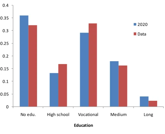
Figure 2 shows the educational distribution of partners for individuals with a vocational

education. The SBAM algorithm finds it necessary to move the distribution slightly to

ensure that the over-all matching is solved. In comparison to the original data, the

pro-portions of partners with educational levels of “High school” and “Vocational” have thus

fallen, while the proportions of “No education”, “Medium” and “Long” have risen.

Figure 3 displays the regional distribution of partners for individuals living in

“Copen-hagen, environs”. The Copenhagen area is divided into two regions: “Copen“Copen-hagen,

envi-rons” (7) and “Copenhagen, city” (6). It is seen that approximately 50 per cent of new

partners also live in the environs of Copenhagen. In addition, Copenhagen city and North

Sealand (8) account for a significant proportion of new partners. It is evident that the

SBAM method produces a distribution that is fairly consistent with the original data.

Figure 4 shows the distribution of matchings on the age difference. There is a significant

change in the age-difference distribution as the matching ages, such that young couples

tend to have a more lower age difference compared to later on in their life. When they

Figure 1: Age distribution of partners. 25-29 year old males.

Ϭ Ϭ͘ϬϮ Ϭ͘Ϭϰ Ϭ͘Ϭϲ Ϭ͘Ϭϴ Ϭ͘ϭ Ϭ͘ϭϮ

ϭϱ ϮϬ Ϯϱ ϯϬ ϯϱ ϰϬ ϰϱ

ŐĞ

ϮϬϮϬ

ĂƚĂ

Source: Own calculations.

Figure 2: Educational distribution of partners. Vocational (?).

Ϭ Ϭ͘Ϭϱ Ϭ͘ϭ Ϭ͘ϭϱ Ϭ͘Ϯ Ϭ͘Ϯϱ Ϭ͘ϯ Ϭ͘ϯϱ Ϭ͘ϰ

EŽĞĚƵ͘ ,ŝŐŚƐĐŚŽŽů sŽĐĂƚŝŽŶĂů DĞĚŝƵŵ >ŽŶŐ

ĚƵĐĂƚŝŽŶ

ϮϬϮϬ

ĂƚĂ

Figure 3: Regional distribution of partners. Copenhagen, environs.

Ϭ Ϭ͘ϭ Ϭ͘Ϯ Ϭ͘ϯ Ϭ͘ϰ Ϭ͘ϱ Ϭ͘ϲ

ϭ Ϯ ϯ ϰ ϱ ϲ ϳ ϴ ϵ ϭϬ ϭϭ

ZĞŐŝŽŶ

ϮϬϮϬ

ĂƚĂ

Note: Copenhagen, city=6, Copenhagen, environs=7, North Sealand=8.

Source: Own calculations.

6 Conclusions

Most current microsimulation models are based upon a sample of individuals from the

population, which limits the computational requirements in the matching process which is

usually a quadratic complexity process and thus would increase quadratic as the sample

size increases. Few models exceeds a sample size above 100.000 individuals which would

imply a matching pool of approximately 2.500 persons. This low sample size is problematic

when distributing the simulated population on a larger number of characteristics and limit

the fineness of the distribution. This has invoked the modellers to apply rather coarse

methods which does not allow matching distributions to vary with the age-level only the

age-difference, improvements have been imployed by allowing for a distinction between

Figure 4: Distribution age-difference matching, historic vs. estimated

Note: Solid lines are estimated shares, while dotted lines are observed. Data is from the period 2001-2008. The horisontal vertex is the age difference of a matching couple. Source: Own calculations.

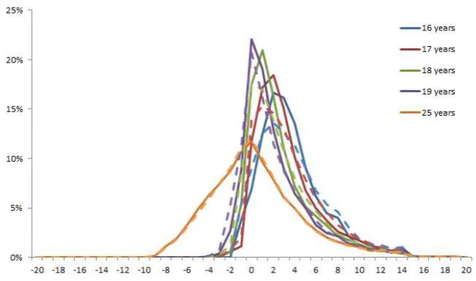
Figure 5: Age difference distribution, young ages

Note: The probability of a person of a given age is matched with a person of a given age-difference. Solid lines are adjusted, dotted lines are observed.

Figure 6: Distribution on education

Note: The probability of a person matched in 2006 with a match of a given education. Source: Own calculations

Figure 7: Distribution on geographical region

Note: The categories are: Copenhagen city, Copenhagen suburb, Northern sealand, Bornholm, Eastern sealand, Western/southern sealand, Fyn, Southern Jutland, Eastern jutland, Western jutland, Northern jutland. The probability that a person matching a person in 2006 is matched with a person in a given region.

this approach arises due to the male-centric assumption.

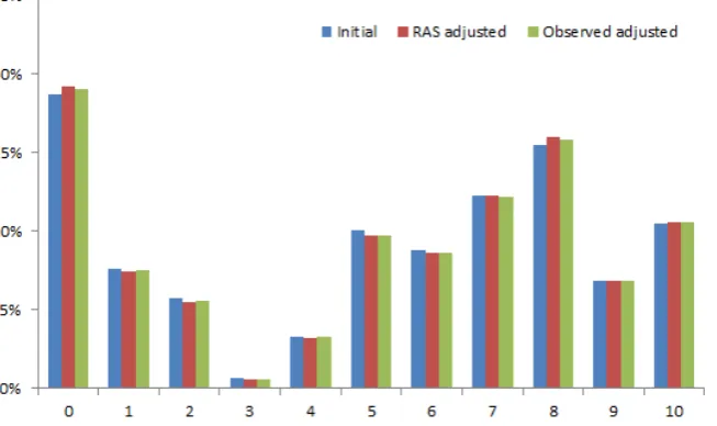
We introduce a new method for computational efficient matching based on the RAS

method of rebalancing matrices and the linked-lists method of C#. Overall the method

mimics the stable approach emencing from changes in population distributions establishing

the theoretical fundation on solid consistent grounds while retaining the observed

distri-bution, which is often a problem for stable approaches that tends to produce bimodal

distributions that cluster too much around the center of the distribution. On the other

hand the method is rather efficient in its computational requirements.

Applications of the method to the historical period 2001-2009 of observed matchings

compared with the SBAM method reveals that the method in general perform very well in

predicting the distribution on age differentials while the most serious errors are observed

7 References

(1) McDougall, Robert A. (1999) ”Entropy Theory and RAS are Friends”. GTAP Working Paper 5-14-1999

(2)

Bregman, Lev M. (1967) “Proof of the convergence of Sheleikhovskii’s method

for a problem with transportation constraints”, USSR Computational

mathematics and mathematical Physics, 1(1), 191-204, 1967.

(3) Gale, D. and Shapley, L. (1962) “College admissions and the stability of marriage”, American Mathematical Monthly 69, pp. 9-14

(4)

Schneider, Michael H. and Zenios, Stavros A. (1990) “A Comparative Study of

Algorithms for Matrix Balancing”. Operations Research, Vol. 38, No. 3 (May

-Jun., 1990), pp. 439-455.

(5) Choo, E. & Siow, A. (2006), “Who marries whom and why”, Journal of Political Economy vol .114, No. 1, pp. 175-201

(6) Shannon, C.E. (1948) “A mathematical theory of communication”. Bell System Technical Journal, 27:379–423, 623–659.

(7) Schoen, Robert (1988) “Modeling multigroup populations”, Plenum Press, New York

(8) Kristensen Joakim B. (2011) “Det danske boligmarked i 2000’erne - kortlægning af boligbestand og flyttebevægelser”, DREAM working paper 2011:3.