Particle Markov Chain Monte Carlo Techniques of Unobserved Component Time Series Models Using Ox

Munich Personal RePEc Archive

Particle Markov Chain Monte Carlo

Techniques of Unobserved Component

Time Series Models Using Ox

Nonejad, Nima

1 May 2014

Online at

https://mpra.ub.uni-muenchen.de/55662/

Particle Markov Chain Monte Carlo Techniques of

Unobserved Component Time Series Models Using Ox

Nima Nonejad

Aarhus University and CREATES

Abstract

This paper details particle Markov chain Monte Carlo (PMCMC) techniques for analysis of

un-observed component time series models using several economic data sets. PMCMC provides a

very compelling, computationally fast and efficient framework for estimation and model

com-parison. For instance, we estimate a stochastic volatility model with leverage effect and one

with Student-t distributed errors. We also model time series characteristics of US inflation

rate by considering a heteroskedastic ARFIMA model where heteroskedasticity is specified by

means of a Gaussian stochastic volatility process.

Keywords:Bayes, Metropolis-Hastings, Particle filter, Unobserved components (JEL:C11, C22, C63)

∗_{The author acknowledges support from CREATES-Center for Research in Econometric Analysis of Time Series}

1

Introduction

In this article we analyze different economic data sets using particle Markov chain Monte Carlo

(PMCMC) techniques, see Andrieu et al. (2010) implemented in Ox (Doornik 2009). The aim

of this paper is not to focus on the properties of PMCMC nor to provide thorough analysis of

empirical data. Instead, we aim to describe the basic steps of PMCMC together with details on

implementation of some of the key algorithms in Ox. These algorithms are chosen for the insights

that they provide. They are not always the most advanced or quickest way of programming in

Ox. Rather, we show that Ox provides a very compelling and computationally fast framework for

estimating rather advanced econometric models. We illustrate these methods on three problems, producing rather generic methods.

The main difference between MCMC and PMCMC is that where in traditional MCMC, in

particular Gibbs sampling problems we resort to converting nonlinear or non-Gaussian models to

linear and Gaussian state space models in order to draw the latent states, in the PMCMC framework

we integrate these latent states out directly using the particle filter and thereafter sample the model

parameters using Metropolis-Hastings. This is due to the results in Andrieu et al. (2010) where they

show that when an unbiasedly estimated likelihood is used inside a Metropolis-Hastings algorithm

then the estimation error makes no difference to the equilibrium distribution of the algorithm. We

believe that applying the PMCMC methodology to unobserved component models is in fact the most important contribution that we make. As we shall see for these type of models, PMCMC

requires limited design effort on the user’s part especially if one desires to change some features

in a particular model. It allows us straightforwardly to develop a sampling algorithm by changing

only few lines in our codes. On the other hand, estimating the same type of models using “pure”

Gibbs sampling would require relatively more programming effort.

We briefly introduce the main concepts of PMCMC in section 2. The initial model in Section

3 is the standard stochastic volatility (SV) model with Gaussian errors applied to a financial data

set concerning daily OMXC20 returns. Next, we consider different well-known extensions of the

SV model. The first extension is a SV model with Student-t errors. In the second extension we

incorporate a leverage effect by modeling a correlation parameter between measurement and state errors. In the third extension we implement a model that has both stochastic volatility and moving

average errors, see for example Chan (2013). The fourth extension is PMCMC implementation of

the stochastic volatility in mean model of Koopman and Hol Uspensky (2002). In this specification

the unobserved volatility process appears in both the conditional mean and the conditional variance.

Finally, we consider a two factor stochastic volatility model as in Harvey et al. (1994) and Shephard

(1996). We show that PMCMC provides a straightforward procedure for estimation and marginal

marginal likelihood is relatively easy using the method of Gelfand and Dey (1994) as the integrated

likelihood is easily available from the particle filter.

Thereafter, we reconsider the unobserved components model of the US inflation rate, see Stock

and Watson (2007), Grassi and Proietti (2010). We estimate different specifications of the un-observed components model using PMCMC. Model selection is again carried out by comparing

marginal likelihoods between models. Results indicate that the specification in which the volatility

of both the regular and irregular components of inflation evolve according to SV processes performs

best in terms of ML. Finally, we show that it is also relatively easy to estimate more complicated

models using PMCMC. We do this by estimating an autoregressive fractionally integrated moving

average (ARFIMA) model with time-varying volatility modeled as a Gaussian SV process using

monthly postwar US core inflation data from 1960 to 2013.

The main concepts of PMCMC with focus on Metropolis-Hastings and the particle filter are

presented in section 2. In section 3 we present several applications to demonstrate the performance of the algorithms using different economic data sets and finally the last section concludes.

2

Markov Chains and Particle Filters

Consider the simplest formulation of the stochastic volatility (SV) model

yt = exp(αt/2)εt, εt∼N(0,1) (2.1)

αt+1 = µ+φ(αt−µ) +σ ηt, ηt∼N(0,1) (2.2)

whereyt is the observed data,(α1, ...,αT) ′

are the unobserved log-volatilities, µ is the drift in the state equation, σ is the volatility of log-volatility and φ is the persistence parameter. Typically, we would impose that|φ|<1 so that we have a stationary process with the initial condition,α1∼

N µ,σ2_{/ 1−φ}2

. Let θ = µ,φ,σ2′

and YT = (y1, ...,yT) ′

. This model has been heavily

analyzed in time series econometrics, see for example Kim et al. (1998). The major challenge

of estimating this model is that while sampling p(θ |α1, ...,αT,YT) is relatively easy, sampling

α1, ...,αT ∼p(α1, ...,αT |θ,YT)is often difficult.

Within the Gibbs sampling framework, the most popular approach for estimating (2.1)-(2.2)

is the so-called auxiliary mixture sampler, see Kim et al. (1998). The idea is to approximate the

SV model using a mixture of linear Gaussian models. Specifically, we can square both sides of

(2.1) and take the logarithm such that y_t∗=αt+εt∗ wherey∗t =logy2t andεt∗=logεt2. Kim et al.

(1998) show thatε_t∗can be approximated by a seven-component Gaussian mixture density. We can then write this mixture density using an auxiliary random variable,zt ∈ {1, ...,7}that serves as the

mixture component indicator. Hence, ε_t∗|zt∼N mi,s2i

s2_i andωi,i=1, ...,7 are all fixed and given in Kim et al. (1998). Using this approximation the SV

model can be expressed as a linear Gaussian state space model. Bayesian estimation can then be

performed using standard Gibbs sampling techniques for linear Gaussian state space models, see

for instance Kim and Nelson (1999). Finally, notice that using this specification we sample from the augmented posterior, p(θ,α1, ...,αT,z1, ...,zT |YT).

Within the PMCMC framework we need not use the above approximation. On the contrary,

we approach estimating (2.1)-(2.2) directly by first integrating out (α1, ...,αT) ′

and thus obtaining

p(YT |θ)where

p(YT |θ) =

T

∏

t=1

p(yt |Yt−1,θ) (2.3)

In more general cases we do not have a closed form expression forp(yt|Yt−1,θ)and can therefore

only approximate it. In this paper, we use simulations to unbiasedly estimate each term on the

right side of (2.3). This is carried out using the particle filter, see Kim et al. (1998), Doucet

et al. (2000) and Creal (2012). We then use the main result of Andrieu et al. (2010) which states

that when an unbiasedly estimated likelihood is used inside a MCMC algorithm then the estimation

error makes no difference to the equilibrium distribution of the algorithm, the posterior distribution,

p(θ |YT)∝ p(YT |θ)p(θ). Thus, conditional on p(YT |θ)and the prior, p(θ)we can sampleθ

from p(θ |YT)by using Metropolis-Hastings (M-H). M-H follows the steps:

1. Initialize, start with a vector of parameters,θ(0)_{, seti=1.} 2. Draw a candidate valueθ∗∼q

θ |θ(i−1)_.

3. Acceptθ∗with probability

aMH

θ∗,θ(i−1) = min  

 1,

p(θ∗|YT)q

θ(i−1)_|θ∗ p θ(i−1)_|Y

Tq θ∗|θ(i−1)

 



(2.4)

4. Ifθ∗_{is accepted, setθ}(i)_=θ∗_{, elseθ}(i)_=θ(i−1)_. 5. Seti=i+1 and repeat from Step 2.

The candidate density,q

θ |θ(i−1)_{can be chosen freely, though a density which is related to the} target density would lead to better acceptance rates. We start by using the random walk

Metropolis-Hastings algorithm, see Koop (2003). Thus, we generateθ∗fromqθ |θ(i−1)_∼Nθ(i−1)_,Σ

q

where Σ_q is chosen by the researcher in a manner to ensure a sufficient acceptance rate. A

(2003, page 98) and adjust Σ_q to get acceptance rates roughly around 30 to 40%. We do this by

experimenting with different values ofΣ_quntil we find one which yields a reasonable acceptance

rate probability.

To allow for faster convergence and even better mixing we follow So et al. (2005) and do the following: we perform the random walk M-H algorithm for the first N1 of the total N PMCMC

iterations and form the sample mean, ˆθ and sample covariance, ˆΣfor nθ(i)oN1

i=1. Then, using the

Gaussian proposal with mean ˆθ and covariance ˆΣ, we perform the following independent kernel M-H algorithm for the remainingN2=N−N1iterations. Hence,

1. At iterationiwherei≥(N1+1), generateθ∗fromN θˆ,Σˆ

2. Acceptθ∗_{with probability}

aMH

θ∗,θ(i−1) = min  

 1,

p(θ∗|YT)q

θ(i−1)

p θ(i−1)_|Y

T

q(θ∗₎

 



(2.5)

whereqθ(i−1)_{is the Gaussian proposal density with mean ˆθ and covariance ˆΣevaluated} atθ(i−1)_.

3. Seti=i+1 and repeat from Step 2.

Finally, for the SV model we specify the priors for µ,φ andσ2_as

µ ∼N(0,1) , φ+1

2 ∼Beta(20,1.5) , σ

2_∼IG

4 2,

0.02 2

whereIG s0

2,

v0

2

denotes the Inverse-gamma density, see Kim and Nelson (1999).

2.1

Particle filter

The particle filter is a sequential simulation device for filtering of non-Gaussian, nonlinear state

space models. It can be thought of as a generalization of the Kalman filter, which is only able to analyze linear, Gaussian state space models. Both the particle and Kalman filters produce filtered

estimates of(α1, ...,αT) ′

and p(yt |Yt−1,θ)fort=1, ...,T. In the Kalman case all these quantities

are exact whereas in the particle filter case they are simulation-based estimates.

The main idea of the particle filter is to sample a cloud of particles,αt(j), j=1, ...,Msuch that

they together describe the density of the state variable at time t conditional onYt. At each t we

very general particle filter that we use throughout this paper. For more details on particle filtering

the reader is referred to Doucet et al. (2000) and Creal (2012). Our particle filter scheme is as

follows:

1. Sett=1 andl0=0. Drawαt(1), ...,α

(M)

t fromαt|α0,θ.

2. Computeτt(j)=p

yt|αt(j),Yt−1,θ

andw(_tj)=τt(j)/

ΣM k=1τ

(k)

t

for j=1, ...,M.

3. Resample nαt(1), ...,α

(M)

t

o

with probabilities w_t(1), ...,w_t(M). First, draw u∼U(0,1). Let

x(j)= _Mu + (j−1)/M for j=1, ...,M and find indicesi1, ...,iM such thatΣi_kj₌−1₁w(_tk)<x(j)≤

Σi_kj₌₁w(_tk). We refer to this step as the “Resampling step” for future references.

4. Sampleα_t(₊j)₁∼αt+1|α(

ij)

t ,θ for j=1, ...,M.

5. Computelt(θ) =lt−1(θ) +log

M−1ΣM

j=1τ

(j)

t

. Sett =t+1 and goto step 2.

As an estimate forE[αt |α1, ...,αt−1,Yt−1,θ]we use ˆαt =ΣMj=1w

(j)

t α

(j)

t . A basic implementation

of the particle filter is provided in Table 1.

Del Moral (2004, Theorem 7.4.2) shows that p(\YT |θ) =E[exp(lT(θ))] = p(YT |θ).

There-fore, since the particle filter provides us with an unbiased estimate ofp(YT |θ)we can use the result

in Andrieu et al. (2010) and replace p(YT |θ) with p(\YT |θ)inside a MCMC sampling scheme.

Thereafter, we sample θ which has a relatively lower dimension using Metropolis-Hastings. Ba-sic code for evaluating aMH

θ∗,θ(i−1)_{itself could be implemented as in Table 2. The routine}

❢✉♥❝▼❡tr♦♣♦❧✐s❍❛st✐♥❣✭✮ draws θ∗_{, evaluates a} MH

θ∗_,θ(i−1) _{using (2.4) for i=1, ...,N}

1

and (2.5) fori=N1+1, ...,N. Fori=1, ...,N1we specify the random walk variance,Σqas✈t✉♥❡.

As stated before, we experiment with several values for ✈t✉♥❡ in order to get reasonable accep-tance rate probabilities. For insaccep-tance, for the Gaussian SV model we set: △µ(i) _=0.2828ε(i)

1 ,

△φ(i)_=0.01ε(i)

2 and△σ2(i)=0.01ε

(i)

3 whereεk∼N(0,1)fork=1, ...,3. Thereafter, we follow

section 2 and perform independent kernel Metropolis-Hastings for the remainingN2draws.

The function❢✉♥❝P♦st❡r✐♦r✭✮evaluates p(θ∗|YT)asθ∗ is generated. In order to evaluate p(θ∗|YT) we need to run the particle filter usingθ∗. The denominator is evaluated usingθ(i−1)

and p YT\|θ(i−1)

which are available from the previous iteration. We thereafter complete the

M-H step by drawing u from the standard Uniform distribution. IfaMH

θ∗_,θ(i−1)_{≥u we set}

θ(i)_=θ∗ _{and p Y}\

T |θ(i)

= p(\YT |θ∗), else we retainθ(i−1) and p YT\|θ(i−1)

. Thereafter, we

2.2

Bayes factors and marginal likelihood computation

The main output from the particle filter is the loglikelihood contribution of each observation. The

sum of the loglikelihood contributions delivers the estimated loglikelihood of the data, p(\YT |θ),

with the unobserved states integrated out. This quantity can then be used to compute the marginal

likelihood (ML) for a modelM_{. The marginal likelihood is defined as}

p(YT |M) =

ˆ

Θ

p(YT |θ,M)p(θ |M)dθ

In the following steps the model index,M is suppressed for conciseness. Gelfand and Dey (1994)

propose a very compelling and general method to calculate ML. It is efficient and utilizes the

same routines when calculating ML for different models. The Gelfand-Dey (G-D) estimate of the

marginal likelihood is based on

1

N N

∑

i=1

gθ(i)/hpYT |θ(i)

pθ(i)i → p(YT)−1 as N →∞ (2.6)

whereas before, N is the number of PMCMC iterations. G-D show that if gθ(i)_{is thin-tailed} relative to pYT |θ(i)

pθ(i)_{then (2.6) is bounded and the estimator is consistent. Following} Geweke (2005) a truncated Normal distribution, N(θ∗,Σ∗) is used for g(θ). θ∗ and Σ∗ are the posterior sample moments calculated as

θ∗= 1

N N

∑

i=1

θ(i) and Σ∗= 1

N N

∑

i=1

θ(i)−θ∗ θ(i)−θ∗

′

wheneverθ(i) _{is in the domain of the truncated Normal. The domain,Θis defined as}

Θ =

θ : θ(i)−θ∗

′

(Σ∗)−1θ(i)−θ∗≤χ_a2(z)

where z is the dimension of the parameter vector and χ2

a(z) is the ath percentile of the

Chi-squared distribution with z degrees of freedom. In practice, 0.75, 0.95 and 0.99 are popular se-lections for a. Once the marginal likelihood for different specifications has been calculated, we

can compare them using Bayes factors, BF. The relative evidence forM_A versusM_B isBFM_AB = p(YT |MA)/p(YT |MB). This odds ratio is the factor by which the data considersMAmore

prob-able thanM_{B. Kass and Raftery (1995) recommend considering twice the logarithm of the Bayes}

factor for model comparison and suggest a rule-of-thumb of support forM_{A based on 2 logBFM}

AB:

0 to 2 not worth more than a bare mention, 2 to 6 positive, 6 to 10 strong, and greater than 10 as

3

Applications

3.1

Stochastic volatility models

In this section we estimate the standard stochastic volatility (SV) model along with different

ex-tensions. The first of these extensions we label the SVt model whereεt ∼St(v)andSt stands for

the Student-t distribution withv>2 degrees of freedom. In the second extension we incorporate a leverage effect by lettingρ denote the correlation betweenεt andηt. We shall refer to this model as

SVL. Notice that in both cases we need only to make small adjustments in the codes. With regards

to the SVt model, for p(yt|αt,Yt−1,θ)we use

p(yt|αt,Yt−1,θ) =

Γ v+₂1

Γ v₂ p

(v−2)π

1

σt

1+ y

2

t

(v−2)σ2

t

−(v+1)/2

We then follow the sampling steps as before. On the other hand, if we were to use pure Gibbs

sampling to estimate the SVt model then we would be forced to convert the model into a

condition-ally Gaussian state space model by lettingεt=λ

−1/2

t et whereet∼N(0,1)andλt ∼G(v/2,v/2).

We would then follow the steps in Chib et al. (2002) and sample from the augmented posterior,

p(θ,v,α1, ...,αT,z1, ...,zT,λ1, ...,λT |YT) whereas before,zt serves as the mixture component

in-dicator.

For the SVL model we need only to rewrite (2.2) as

αt+1 = µ+φ(αt−µ) +σ ρytexp(−αt/2) +σ

q

(1−ρ2_)ξ

t

Here, we use thatηt=ρεt+

p

(1−ρ2_)ξ

t whereξt ∼N(0,1)and we need to sample an additional

parameter, ρ. We choose the same priors as in section 2 for µ, φ and σ2_{. With regards to the}

additional parameters we letv∼Exp(0.2)whereExpdenotes the Exponential distribution and we setρ ∼N(0,1)truncated such that −1<ρ <1. The prior on ρ assumes thatρ lies between−1 and 1. Furthermore, we ensure that

ρ

(i)

<1 by resamplingρ

(i)_until ρ

(i) <1.

We can also expand the plain stochastic volatility model by allowing the errors in the

measure-ment equation to follow a moving average (MA) process of orderm, see for example Chan (2013).

This means that the errors in the measurement equation are no longer serially independent as for

the plain SV model. Here, we choose a more simple specification and setm=1. Hence, our model is given as

yt = eαt/2εt+ψeαt−1/2εt−1, εt∼N(0,1)

As before, we impose that |φ| <1, α1∼ N µ,σ2/ 1−φ2

and we also ensure that the root

of the characteristic polynomial associated with the MA coefficient, ψ is outside the unit circle. Notice that under the standard stochastic volatility model, the unconditional variance ofytis simply

eαt_{. However, under the moving average variant, the unconditional variance of y}

t is given by eαt_+ψ2_eαt−1_{. Hence, in this case the unconditional variance is time-varying through two channels:}

the moving average term ofeαt _andα

t which evolves according to (2.2). Estimating this model is

straightforward as again we only need to make small adjustments in the codes. With regards toψ, we let p(ψ)∼N(0,1)truncated such that−1<ψ <1.

The flexibility of PMCMC can be used to model other attractive specifications of the stochastic

volatility model. For instance, consider the popular stochastic volatility in mean (SVM) model

of Koopman and Hol Uspensky (2002) where eαt/2 _{appears in both the conditional mean and the}

conditional volatility. We follow the same notation as before and define the SVM model as

yt = βexp(αt/2) +exp(αt/2)εt, εt∼N(0,1)

where αt follows (2.2). Estimation of this extension is nontrivial using pure Gibbs sampling.

This is because drawing α1, ...,αT ∼ p(α1, ...,αT |θ,β,YT) is computationally more

demand-ing since the model cannot be written in linear state space form. However, within the PMCMC

context estimating the SVM model is straightforward. In fact, we note that p(yt |αt,Yt−1,θ)∼

N(βexp(αt/2),exp(αt)). Incorporating this specification is very easy in the particle filter as we

only need to modify step 2 of the algorithm and thus use τ_t(j) =N

βeαt(j)/2,_eα

(j)

t

, j=1, ...,M. Furthermore, in the M-H step we sample an additional parameter,β where p(β)∼N(0,1).

It was suggested to provide a simulation example of SV-MA(1) and SVM. We present

simula-tion results in appendix A where we also experiment with different values of M to see its impact

on the results, especially for low values ofM, for exampleM=1 orM=10. Finally, we estimate a two factor SV model, TFSV. We define TFSV as

yt = exp

µ

2 +

αt+α2t

2

εt, εt ∼N(0,1)

αt = φ αt−1+σ ηt, ηt∼N(0,1)

α2t = φ2α2t−1+σ2η2t, η2t∼N(0,1) |φ|<1 , α1∼N 0,σ2/ 1−φ2

|φ2|<1 , α21 ∼N 0,σ22/ 1−φ22

Estimating the two factor SV model using PMCMC is straightforward. First, we collect all the

parameters in θ = µ,φ,φ2,σ2,σ22

′

. Then, we only need to modify the particle filter such that

easy and does not cost anything in terms of computation. We specify the increments in the M-H

part as △µ(i) =0.3162ε₁(i) whereε₁(i)∼N(0,1). Forφ andφ2 we find that M-H is very sensitive

with regards to their values. Therefore, we try get as close as possible to the center of the posterior.

Hence, we perform the following, see also Fouque et al. (2010): First, we put the restrictionφ>φ2.

This restriction is needed for identification. We then draw φ and φ2 from a truncated Normal

density. For instance,φ∗∼N b,B−1truncated such that|φ∗|<1 whereb= (1/B)ΣT t=1α

(i−1)

t α

(i−1)

t−1

and B=ΣT t=1α

2(i−1)

t−1 1. We draw µ, σ2 and σ22 as before and thereafter accept or reject θ∗. For

the priors, we set µ ∼N(0,1), φ ∼N(0,1), φ2∼N(0,1), truncated such that|φ|<1, |φ2|<1,

σ2_{∼IG(4/2,0.02/2)andσ}2

2 ∼IG(4/2,0.02/2).

The top panel in Figure 1 displays the OMX Copenhagen 20 (OMXC20) index for the period

1/2/2006-12/30/2010 followed by the returns and the filtered estimates of ˆσt=exp(αˆt/2)fort =

1, ...,T. From these figures strong differences in return and volatility are apparent2. For instance, the top left panel shows a sharp decrease in the OMXC20 index towards the end of 2008. At the same time the third panel in the top row of Figure1 shows an increase in the conditional volatility

of SVL for that time period.

We setM=1000 and run our sampler forN=20000 M-H iterations. After discarding the first 10000 iterations we collect the final sample and compute the posterior mean, θ , 95% credibility intervals (indicated inside the brackets), the inefficiency measures,RB, the loglikelihood that results

from the particle filter, the logarithm of the marginal likelihood, log(ML) fora=0.75,a=0.99 and the M-H acceptance ratio. The inefficiency measures display the relative variance of the posterior

sample draws when adapting for correlation between iterations, as compared to the variance without

accounting for correlation. In these calculations, we follow Bos (2011) and choose a bandwidth,B

of 100, see also Kim et al. (1998) for a further background on this measure. Results are summarized

in Table 3.

We find that the Gaussian SVL model performs best in terms of the marginal likelihood

crite-rion3. The 2logBF of SVL versus SV in Table 3 is 7.8 and this indicates strong evidence in favor of the SVL model. Compared to SVt the 2logBF in favor of SVL is 12.8 which is also very strong evidence. The distribution of the parameters,θ = µ,φ,σ2_,ρ′

are also concentrated around their

means. The values of φ close to one confirm strong daily volatility persistence, in accordance with typical estimates reported in the literature. Notice that the persistence increases slightly as

the fat-tailed error distribution is introduced (φ =0.9810 and 0.9852 for the SV and SVt model,

1_{We could also choose aBeta(20,1.5)prior forφ andφ2. However, we find thatφ2is very sensitive with regards} to the hyperparameter values ofBeta(., .). Therefore, we choose a more uninformative prior, i.e. N(0,1)truncated to ensure that|φ|<1.

2_{OMX Copenhagen 20 (OMXC20) is the Copenhagen Stock Exchange’s leading share index. The index consists}

of the 20 most actively traded shares on the Copenhagen Stock Exchange.

3_{An advantage of using Bayes factors is that they automatically include Occam’s razor effect in that they penalize}

respectively) and drops fromφ =0.9810 for SV toφ =0.9777 for SVL. In the SVt model, the dis-tribution of the degrees of freedom parameter is centered around 14.20 with a standard deviation of 2.28. For the SVL model the posterior mean ofρ is−0.22 and negative as expected. We also find thatψ =0.0045 for the SV-MA(1) model. Compared to SV-MA(1) the 2logBF in favor of SVL is 15.8. On the other hand, we estimate β at 0.5636 with a standard deviation of 0.1688. However, compared to SV or SVL, SVM does not offer any improvements in terms of ML. Finally, TFSV

performs worst in terms of ML. The estimates of µ, φ andσ2 _{are relatively close to those for the}

plain SV model. On the other hand, the estimates ofφ2andσ₂2show that the second factor,α2t is

very close to being a white noise process.

In Figure 1 we report the Markov chain output for µ |YT, φ |YT , σ2|YT, ρ |YT along with

histograms and the evolution of ACFs for these parameters. The chain mixes well with relatively

fast decaying autocorrelation functions.

3.2

Unobserved components model of inflation

In this section we reconsider the unobserved components model of Stock and Watson (2007) and

provide a computational framework using PMCMC. This model provides a simple but yet

suffi-cient framework for discussing the main stylized facts concerning inflation. Specifically, the model

postulates the decomposition of observed inflation into two components: the regular component

which captures the trend in inflation and the irregular component which captures the deviations of

inflation from its trend value. We start from a specification where components are driven by

distur-bances whose variance are constant over time. Thereafter, we consider specifications in which the

components are driven by disturbances whose variance evolves over time according to a stationary stochastic volatility process.

We focus on quarterly inflation rates constructed from the seasonally adjusted consumer price

index, made available by Fred (Federal Reserve Economic Data). We denote the quarterly

se-ries by CPIt. The annualized quarterly inflation rate, denoted yt, t = 1, ...,T is computed as yt =400 log(CPIt/CPIt−1). For the analysis we use data from 1952:q1-2013:q1. In the

follow-ing the most general specification of the unobserved component (UC) model is defined as

yt = αt+εt, εt ∼N 0,σε2

(3.1)

αt+1 = αt+ηt, ηt ∼N 0,ση2

(3.2)

This model contains two parameters,θ= σ2 ε,ση2

′

and a vector of the unobserved states,(α1, ...,αT) ′

.

We letp σ2 ε

∼IG 4₂,0.₂02

andp σ2 η

∼IG 4₂,0.₂02

. PMCMC implementation of this model

routine is presented in Table 4.

We also provide extensions of (3.1) and (3.2) by incorporating stochastic volatility effects inσ2 ε

or both inσ2

ε andση2. First, leth1t=logσε2t where

h1t+1 = µ1+φ1(h1t−µ1) +σ1η1t, η1t ∼N(0,1)

Hence, in this case we add a second unobserved state which describes the evolution of the

log-volatility to the irregular component of inflation. We shall refer to this model as UC-SVm. Finally,

we add a third unobserved state which describes the log-volatility of αt. Henceforth, we refer to

this model as UC-SV4.

UC-SVm and UC-SV both have a special structure. For instance, for the UC-SV model, condi-tional onhkt,k=1,2 the remaining model is a linear Gaussian state space model where(α1, ...,αT)

′

can be integrated out analytically using the Kalman filter. This is known as Rao-Blackwellization

in the literature because it is an implication of the Rao-Blackwell Theorem, see Robert and Casella

(2004). When this is possible, the state vectors can be separated. Particles are only simulated for

h(_ktj) k=1,2 and conditional on these we can integrate αt, t =1, ...,T out analytically using the

prediction and updating steps of the Kalman filter.

In the PMCMC procedure we modify the particle filter using the approach of Creal (2012). In

the following we provide the steps of the modified particle filter for the UC-SV model.

1. Fort=1, drawα₁(1), ...,α₁(M),P₁(1), ...,P₁(M)wherePt is the covariance ofαtand it is obtained

from the Kalman filter, see Kim and Nelson (1999). Drawh(_k1₁), ...,h_k(M₁) fork=1,2 and set

τ₁(1), ...,τ₁(M)=1/M.

2. fort =2, ...,T use the prediction step of the Kalman filter and obtain prediction errors and variances,nv(_tj),f_t(j)oM

j=1.

3. Computeτt(j)∼N

v_t(j),f_t(j)and normalizew_t(j)=τt(j)/ΣMk=1τ

(k)

t .

4. Resample M particles with probabilitiesw(_t1), ...,w_t(M) using the “Resampling step” and set

w(_tj)=1/M.

5. Drawh(_kt1), ...,h_kt(M), k=1,2 and run the updating step of the Kalman filter on each of these particles to obtainnαt(j),P

(j)

t

oM

j=1.

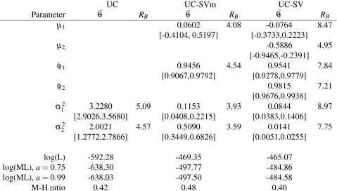
Finally, we compare the performance of UC, UC-SVm and UC-SV using the marginal likelihoods.

The implementation of G-D for the UC model is provided in Table 5. Notice that calculating the

4_{The specification of the stochastic volatility processes differs only slightly from Stock and Watson (2007) who}

marginal likelihood of UC-SVm or UC-SV is very straightforward. Results, reported in Table 6,

point out that with regards to ML the UC-SV model performs best.

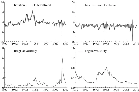
The filtered estimate of(α1, ...,αT) ′

and the filtered estimates of the volatilities are all available

from the particle filter. They are pictured in Figure 2 together with yt. These estimates confirm

largely the results of Stock and Watson (2007) and Grassi and Proietti (2010). The volatility of

the irregular component, exp(h1t/2) increases during the high periods of inflation in the 1970s,

while the volatility of the regular component, exp(h2t/2) is relatively more stable. Specifically,

exp(h2t/2) has been decreasing substantially after 1982. The decrease in exp(hkt/2), k =1,2

since the early 1980s and throughout the 1990s has been documented in a range of studies and it is

often labeled “The Great Moderation”. Finally, exp(h1t/2)shows that the increase in volatility of

the inflation rate during the last recession is mainly concentrated in the irregular component.

3.3

Long memory with stochastic volatility

In this section we model changing time series characteristics of monthly US core inflation rate by

considering a heteroskedastic ARFIMA model similar to Bos et al. (2012). The heteroskedasticity

is specified by a Gaussian SV process, see section 2.

The ARFIMA(0,d,0) model for a time series,yt with time-varying volatility,σεt,t=1, ...,T is

given by

(1−L)d(yt−τ) = σεtεt, εt∼N(0,1) (3.3)

The fractional difference operator(1−L)dwithd∈Ris given by

(1−L)d =

∞

∑

j=0

d

j

!

(−L)j

Here, we assume that 0<d <0.5 and specify σεt =exp(αt/2) where αt evolves according to

(2.2). We letθ = τ,d,µ,φ,σ2′

and proceed in a very similar fashion as in section 3.1. For the

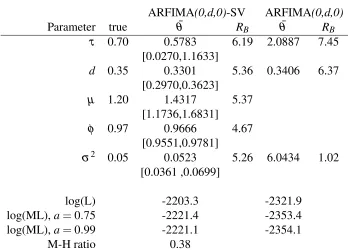
priors ofτ andd we specify p(τ)∼N(0,1)and p(d)∼N(0,1)truncated such that 0<d<0.5. We simulate a data set ofT =1000 observations. We setτ =0.7,d=0.35, µ =1.2,φ =0.97 andσ2_{=0.05. We first generate the volatility sequence according to (2.2) withα}

1∼N µ,σ2/ 1−φ2

.

Thereafter, we use exp(αt/2)εt and generate yt through ARFIMA dynamics usingd and τ. We

estimate (3.3) using PMCMC and compare the estimates with the true parameters. For

compari-son, we also estimate a plain ARFIMA model using Gibbs sampling. Results are summarized in Table 7. Overall, PMCMC works very well as parameter estimates are close to their respective true

We then apply our model to a monthly time series of inflation, using the core consumer price

index (CPILFESL) downloaded from FRED’ s database. This series excludes the direct effects of

price changes for food and energy and it is seasonally adjusted. We denote the price index byPt.

From this price index series, we construct the monthly US core inflation asyt =100 log(Pt/Pt−1).

It can be interpreted as the percentage price change per month. Our series starts in 1960:1 and runs

until 2013:4, for a total of 639 months.

We estimate (3.3) along with an ARFIMA(1,d,0)-SV model. We also estimate an ARFIMA

(1,d,1)-SV model (not reported) but do not find the MA coefficient to be significantly different from zero.

For further comparison we also estimate a homoscedastic ARFIMA(0,d,0)model using Gibbs

sam-pling. Results are summarized in Table 8. For ARFIMA(0,d,0)-SV the order of integration, d, is

estimated at 0.35 and significantly different from 0. This implies that US core inflation exhibits long memory behavior. The average inflation rate, τ is estimated at 0.13% per month. When we estimate an additional parameter, namely, ρ in the ARFIMA(1,d,0)-SV model we find thatd in-creases from 0.35 to 0.46. At the same time the AR coefficient, ρ is estimated at −0.28 and is significantly different from zero. The stochastic volatility component itself is nearly nonstationary

as the autoregressive coefficient of volatility, φ, is close to one and the conditional volatility of volatility,σ is well-identified and estimated at 0.14. The average volatility, exp(µ/2)is at 0.18% per month for both models

The marginal likelihood criterion shows that there is strong evidence in favor of

ARFIMA-SV specifications. The 2 logBF in favor of ARFIMA(0,d,0)-SV compared to ARFIMA(0,d,0) is

212.12. We note further improvements in terms of ML for the ARFIMA(1,d,0)-SV model. We plot the inflation rate along with the filtered estimates of exp(αt/2)for ARFIMA(1,d,0)-SV in Figure 3.

The volatility decrease in the early 1980s is noticeable and persistent. As stated in section 3.2, this

period is labeled as the Great Moderation. We report the Markov chain output ford|YT andρ |YT

along with the evolution of ACFs for these parameters in the bottom rows of Figure 3. Clearly, the

Markov chain mixes well with relatively fast decaying autocorrelation functions.

We also perform a recursive out-of-sample forecasting exercise to evaluate the performance

of ARFIMA-SV models. For each model in Table 9 we produce h-month-ahead point forecasts

with h=1, h=4 and h=8 using a rolling window with a width of 200 months. We choose the out-of-sample period from 1976:9 to the end of the sample for a total of 439 observations.

Specifically, givenYt, t ≥200 we implement our sampling scheme, obtain posteriors draws ofθ

and compute E[yt+h|Yt] using at each steph=2, ...previously obtained forecasts until h-1. As

a new observation enters the information set, the posterior is updated through a new round of

sampling and the forecasting procedure is implemented.

Table 9 reports mean absolute error (MAE) and root mean squared error (RMSE) for the

ARMA(1,1), ARFIMA(0,d,0)and ARFIMA(1,d,0)are estimated using Gibbs sampling.

Overall, we find that ARFIMA(1,d,0)-SV performs very well against the other models. It is

the top performer for h=4, h=8 in terms of MAE and RMSE. For instance, the RMSE of the ARFIMA(1,d,0)-SV model is 10% lower than the RMSE of the AR(1)model for h=1, 23% for

h=4 and 27% forh=8. ARFIMA(1,d,0)-SV also offers improvements in terms of out-of-sample point forecasts compared to ARFIMA(1,d,0). However, these improvements are relatively modest.

In order to perform a joint evaluation of the forecasts and find out if ARFIMA-SV models

generate significant improvements in terms of forecasting the methodology of Hansen et al. (2011),

termed the Model Confidence Set (MCS) is applied. The appealing feature of the MCS approach

is that it allows for a user-defined criterion of “best” and does not require a benchmark model for

comparison. Overall, we see that ARFIMA-SV specifications perform very well compared to their

homoscedastic counterparts and the AR models. Both models belong to the 5% MCS for h=1 while ARFIMA(1,d,0)-SV is the only model that belongs to the 5% MCS forh=4 andh=8, i.e. ARFIMA(1,d,0)-SV performs significantly better than all the other models.

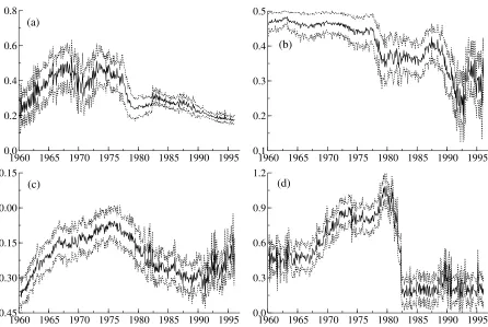
Finally, in order to get a better understanding of changes in the dynamics of US inflation we

follow Bos et al. (2012) and perform a sensitivity analysis using rolling estimates (with a width of

200 months) of the parameters for the ARFIMA(1,d,0)-SV model. We show recursive estimates

of τ, d, ρ and the unconditional volatility of volatility of inflation, pσ2_/1−φ2 _{along with their}

respective one-standard-error credibility intervals in Figure 4. The values for 1960:1 correspond to

the estimation period 1960:1-1976:8.

Panel (a) shows a clear structural break inτ. Recursive estimates ofτfluctuate around 0.35 and 0.4 until the early 1980s and thereafter drop to about 0.25 fluctuating around this value till the end of the sample. More importantly, post-break estimates of τ are relatively more stable confirming a certain degree of success in achieving long run inflation stability since the Great Moderation.

Recursive estimates of d in panel (b) show that d gradually drops from 0.45 at the start of the sample to about 0.3 towards the end of the sample. The estimate ofdis 0.31 for the last subsample which runs from 1996:9 to 2013:4. It is cautiously evident that long memory characteristics of

inflation might not have remained significant after the Great Moderation as evidenced by a smaller

d. On the other hand, ρ increases from−0.4 to−0.1 and then subsequently falls back to around

−0.3 after the Great Moderation until around 1995. Finally, we find a significant one time drop in p

σ2_/1−φ2_{in the beginning of the 1980s confirming the effects of the Great Moderation also in}

4

Conclusion

In this paper we present algorithms and implementations for analyzing different data sets using Ox

in combination with PMCMC techniques. We provide some short Ox programs that show how to

implement the main part of PMCMC. These programs can easily be extended to different models.

In section 3 we provide several empirical examples. We show how to estimate stochastic

volatil-ity models with different specifications. Thereafter, we focus on estimating the unobserved

com-ponents model with time-varying volatility for US inflation data using PMCMC. Results using

quarterly inflation data show that extending the unobserved components model towards a model

with time-varying volatility both in the irregular and regular component of inflation provides im-provements in terms of the marginal likelihood. Finally, we estimate two heteroskedastic ARFIMA

models where heteroskedasticity is specified by a Gaussian SV process. We apply these

mod-els to the monthly US core inflation data from 1960:1 to 2013:4. We find that US core inflation

exhibits long memory behavior. Comparing the ARFIMA-SV models with their homoscedastic

counterparts using the marginal likelihood criterion shows that there is strong evidence in favor of

the ARFIMA-SV models. Sensitivity analysis using rolling estimates of the parameters provides

a clear distinction between parameter changes in the level, long run dynamics and changes in the

References

[1] Andrieu, C., and A. Doucet. 2002. “Particle filtering for partially observed Gaussian state

space models.”Journal of the Royal Statistical Society B 64(4): 827-836.

[2] Andrieu, C., A. Doucet, and R. Holenstein. 2010. “Particle Markov chain Monte Carlo

meth-ods (with discussion).”Journal of the Royal Statistical Society B 72(3): 1-33.

[3] Baillie, R. T., C. F. Chung, M. A. Tieslau. 1996. “Analysing inflation by the fractionally

integrated ARFIMA-GARCH model.”Journal of Applied Econometrics 11(1): 23-40.

[4] Beran, J. 1994.Statistics for Long-Memory Processes. Chapman and Hall.

[5] Bos, C. S. 2011. “A Bayesian Analysis of Unobserved Component Models Using Ox.”Journal

of Statistical Software 41(13): 1-24.

[6] Bos, C. S. 2013.GnuDraw. URL http://www.tinbergen.nl/~cbos/gnudraw.html.

[7] Bos, C. S., S. J. Koopman, and M. Ooms. 2012. “Long memory with stochastic variance

model: A recursive analysis for U.S. inflation.”Computational Statistics and Data Analysis,

forthcoming.

[8] Chan, J. 2013. “Moving Average Stochastic Volatility Models with Application to Inflation Forecast.”Journal of Econometrics 176(2): 162-172.

[9] Chib, S., E. Greenberg. 1995. “Understanding the Metropolis-Hastings Algorithm.” The

American Statistician 49(4): 327-335.

[10] Chib, S., F. Nadari, and N. Shephard. 2002. “Markov chain Monte Carlo methods for

stochas-tic volatility models.”Journal of Econometrics 108(2): 281-316.

[11] Creal, D. 2012. “A survey of sequential Monte Carlo methods for economics and finance.”

Econometric Reviews 31(3): 245-296.

[12] Del Moral, P. 2004.Feynman-Kac Formulae: Genealogical and Interacting Particle Systems

with Applications. Springer.

[13] Doornik, J. A. 2009. An Object-Oriented Matrix Language Ox 6. Timberlake Consultants

Press.

[14] Doucet, A., S. J. Godsill, and C. Andrieu. 2000. “On sequential Monte Carlo sampling

[15] Flury, T., and N. Shephard. 2011. “Bayesian inference based only on simulated likelihood:

particle filter analysis of dynamic economic models.”Econometric Theory 27(5): 933-956.

[16] Gelfand, A., and D. Dey. 1994. “Bayesian Model Choice: Asymptotics and Exact

Calcula-tions.”Journal of the Royal Statistical Society B 56(3): 501-514.

[17] Geweke, J. 2005.Contemporary Bayesian Econometrics and Statistics.Wiley.

[18] Grassi, S., and T. Proietti. 2010. “Has the Volatility of U.S. Inflation Changed and How?”

Journal of Time Series Econometrics 2(1): Article 6.

[19] Hansen, P. R., A. Lunde, and J. M. Nason. 2011. “The Model Confidence Set.”Econometrica

79(2): 453-497.

[20] Jacquier, E., N. G. Polson, and P. E. Rossi. 1994. “Bayesian Analysis of Stochastic Volatility

Models.”Journal of Business & Economic Statistics 12: 371-417.

[21] Kass, R. E., and A. E. Raftery. 1995. “Bayes Factors.” Journal of the American Statistical

Association 90: 773-795.

[22] Kim, C. J., and C. R. Nelson. 1999.State Space Models with Regime Switching Classical and

Gibbs Sampling Approaches with Applications. MIT Press.

[23] Kim, S., N. Shephard, and S. Chib. 1998. “Stochastic Volatility: Likelihood Inference and

Comparison with ARCH Models.”Review of Economic Studies 65(3): 361-393.

[24] Koop, G. 2003.Bayesian Econometrics. John Wiley & Sons Ltd.

[25] Koopman, S. J., and E. H. Uspensky. 2002. “The stochastic volatility in mean model:

em-pirical evidence from international stock markets.” Journal of Applied Econometrics 17(6):

667-689.

[26] Liu, J. S., and R. Chen. 1998. “Sequential Monte Carlo Methods for Dynamic Systems.”

Journal of the American Statistical Association 93(443): 1032-1044.

[27] Pitt, M. K., and N. Shephard. 1999. “Filtering via Simulation: Auxiliary Particle Filters.”

Journal of the American Statistical Association 94: 590-599.

[28] So, M. K. P., C. W. S. Chen, and M. Chen. 2005. “A Bayesian Threshold Nonlinearity Test

for Financial Time Series.”Journal of Forecasting 24(1): 61-75.

[29] Stock, J. H., and M. W. Watson. 2007. “Why Has U.S. Inflation Become Harder to Forecast?”

A

Appendix

In this appendix we present simulation results for SV-MA(1) and SVM. We simulate T =1000 observations from these models and report the true DGP parameters along with PMCMC parameter

estimates in Table 10. In each case we also estimate a plain SV model for comparison. Overall, we

see that PMCMC works very well as parameter estimates are close to their respective true values.

Not surprisingly, in each case the corresponding model outperforms the plain SV model in terms

of ML.

Finally, we analyze the performance of PMCMC with respect to the number of particles, M.

We do this by estimating SV-MA(1) usingM=1,M=10,M=100 andM=1000. In all of these cases we choose N=20000. From the columns of Figure 5 we see that using very low values of

M appears to be insufficient. For instance, forM=1 the chain gets stuck on a specific parameter value almost throughout the sample. ForM=100 we get better results but we still see that the chain gets stuck for a considerable time. However, we see drastic improvements in the performance of

Table 1: The particle filter in Ox

❢✉♥❝P❛rt✐❝❧❡❋✐❧t❡r✭❝♦♥st ✈❤♣❢✱ ❝♦♥st ✈❊❙❙✱ ❝♦♥st ✈❧♦❣♣❞❢✱ ❝♦♥st ✈♣❛r❛♠✱ ❝♦♥st ✈②✱ ❝♦♥st ✐◆✮

④

✳✳✳

✈✇❂♦♥❡s✭✐◆✱✶✮✯✭✶✴✐◆✮❀

✈❧♦❣♣❞❢❬✵❪❬✵❪❂✵❀ ✴✴ ◆♦ ❧✐❦❡❧✐❤♦♦❞ ❝♦♥tr✐❜✉t✐♦♥

❬✈❤❪❂❢✉♥❝■♥P❛rt✐❝❧❡s✭✈♣❛r❛♠✱✐◆✮❀ ✴✴ ■♥✐t✐❛❧ ♣❛rt✐❝❧❡s ❢♦r✭✐❂✶❀ ✐❁✐t❀ ✐✰✰✮

④

✈❆❂❢✉♥❝❘❡s❛♠♣❧❡✭✈✇✬✱✐◆✮❀ ✴✴ ❘❡s❛♠♣❧❡

✈❤❂❢✉♥❝❉r❛✇P✭✈❤❬✈❆✬❪✱✈♣❛r❛♠✱✈②❬✐❪❬✵❪✱✐◆✮❀ ✴✴ ❉r❛✇ ❢r♦♠ q✭✮ ✈❊❂✈②❬✐❪✳✴✭❡①♣✭✵✳✺✯✈❤✮✮❀

✈t❛✉❂❡①♣✭✲✵✳✺✳✯✈❤✮✳✯❞❡♥s♥✭✈❊✮❀ ✴✴ ❈♦♠♣✉t❡ ❧✐❦❡❧✐❤♦♦❞ ✈❧♦❣♣❞❢❬✵❪❬✐❪❬✵❪❂❧♦❣✭♠❡❛♥❝✭✈t❛✉✮✮❀ ✴✴ ❚❛❦❡ ❧♦❣s ✈✇❂✈t❛✉✳✴s✉♠❝✭✈t❛✉✮❀ ✴✴ ◆♦r♠❛❧✐③❡

✐❢ ✭✐s♠✐ss✐♥❣✭✈✇✮✮ ✴✴ ❘❡s❡t ✇❡✐❣❤ts ✐❢ ♠✐ss✐♥❣ ✈✇❂♦♥❡s✭✐◆✱✶✮✴✐◆❀

✈❤♣❢❬✵❪❬✐❪❬✵❪❂s✉♠❝✭✈✇✳✯✈❤✮❀ ✴✴ ❙t♦r❡ ♠❡❛♥ ✈❊❙❙❬✵❪❬✐❪❬✵❪❂✶✴s✉♠❝✭✈✇✳❫✷✮❀ ✴✴ ❙t♦r❡ ❊❙❙ ✐❢✭✈❊❙❙❬✵❪❬✐❪❬✵❪❁✵✳✺✯✐◆✮

④

✴✴ ■❢ ✈❊❙❙❬✵❪❬✐❪❬✵❪❁✵✳✺✯✐◆ r❡s❛♠♣❧❡ ✈❆❂❢✉♥❝❘❡s❛♠♣❧❡✭✈✇✬✱✐◆✮❀

✈❤❂❢✉♥❝❉r❛✇P✭✈❤❬✈❆✬❪✱✈♣❛r❛♠✱✈②❬✐❪❬✵❪✱✐◆✮❀ ✈✇❂♦♥❡s✭✐◆✱✶✮✯✭✶✴✐◆✮❀

⑥ ⑥

Table 2: PMCMC scheme in Ox

❢✉♥❝▼❡tr♦♣♦❧✐s❍❛st✐♥❣s✭❝♦♥st ♠♣r✐♦r✱ ❝♦♥st ✈②✱ ❝♦♥st ✈♣❛r❛♠♦✱ ❝♦♥st ✈♣❛r❛♠q✱

❝♦♥st ♠❝♦✈✱ ❝♦♥st ❞❧♦❣♣❞❢♦✱ ❝♦♥st ✐◆✱ ❝♦♥st ✐❞✉♠t❤✮ ④

✳✳✳

❬✈♣❛r❛♠♣❪❂❢✉♥❝❉r❛✇♣❛r❛♠✭✈♣❛r❛♠q✱♠❝♦✈✱✐❞✉♠t❤✮❀ ✴✴ ❉r❛✇ t❤❡ ❝❛♥❞✐❞❛t❡✱ ✈♣❛r❛♠♣

❬❞♥✉♠✱❞❞❡♥✱❞❧♦❣♣❞❢♣❪❂

❢✉♥❝P♦st❡r✐♦r✭✈♣❛r❛♠♣✱✈♣❛r❛♠♦✱❞❧♦❣♣❞❢♦✱✈②✱♠❝♦✈✱♠♣r✐♦r✱✐◆✮❀

✐❞✉♠❂✵❀

✈♣❛r❛♠♥❡✇❂✈♣❛r❛♠♦❀ ✴✴ ✈♣❛r❛♠♦ ✐s t❤❡ ♦❧❞ ✈❛❧✉❡ ❞❧♦❣♣❞❢♥❡✇❂❞❧♦❣♣❞❢♦❀

✴✴ Pr❡♣❛r❡ t❤❡s❡ q✉❛♥t✐t✐❡s

✴✴ ❙❡t t❤❡ ♥❡✇ ♣❛r❛♠❡t❡rs ❡q✉❛❧ t♦ t❤❡ ♦❧❞ ✴✴ ■❢ ❞❛❧♣❤❛❃❞✉ t❤❡② ✇✐❧❧ ❜❡ r❡♣❧❛❝❡❞

❞❛❧♣❤❛❂♠✐♥✭✶✱❡①♣✭❞♥✉♠✲❞❞❡♥✮✮❀ ✴✴ ❈❛❧❝✉❧❛t❡ ❛▼❍ ❞✉❂r❛♥✉✭✶✱✶✮❀ ✴✴ ❉r❛✇ ❛ r❛♥❞♦♠ ✉♥✐❢♦r♠ ♥✉♠❜❡r ✐❢ ✭❞❛❧♣❤❛❃❞✉✮ ✴✴ ❛❝❝❡♣t

④

✈♣❛r❛♠♥❡✇❂✈♣❛r❛♠♣❀ ❞❧♦❣♣❞❢♥❡✇❂❞❧♦❣♣❞❢♣❀

✐❞✉♠❂✶❀ ✴✴ ❈♦✉♥t t❤❛t t❤❡ ❞r❛✇ ✇❛s ❛❝❝❡♣t❡❞ ⑥

Table 3: Estimation results, stochastic volatility models

SV SVt SVL SV-MA(1) SVM TFSV

Parameter θ¯ θ¯ θ¯ θ¯ θ¯ θ¯

µ 0.3526 (7.54) 0.2562 (7.38) 0.4221 (6.89) 0.3779 (7.78) 0.3754 (7.43) 0.3598 (6.23) [0.1112,0.5895] [-0.0482,0.5508] [0.2046,0.6436] [0.0831,0.6703] [0.0685,0.6708] [0.0821,0.6332]

φ 0.9810 (8.27) 0.9852 (5.33) 0.9777 (6.97) 0.9817 (8.86) 0.9805 (9.63) 0.9776 (7.13) [0.9743,0.9887] [0.9783,0.9914] [0.9716,0.9838] [0.9730,0.9893] [0.9727,0.9882] [0.9671,0.9881]

φ2 0.0458 (10.66)

[-0.0642,0.1576]

σ2 _{0.0296 (9.13) 0.0221 (6.11) 0.0319 (7.36) 0.0285 (7.97) 0.0311 (9.16) 0.0373 (6.59)} [0.0199,0.0394] [0.0149,0.0297] [0.0231,0.0401] [0.0183,0.0395] [0.0203,0.0421] [0.0236,0.0512]

σ2

2 0.0981 (6.31)

[0.0276,0.1728]

ρ -0.2216 (7.04)

[-0.3202,-0.1226]

ψ 0.0045 (7.63)

[-0.0296,0.0376]

β 0.0563 (6.37)

[0.0223,0.0892]

v 14.2019 (8.06)

[9.9591,18.8712]

log(L) -2113.6 -2114.2 -2106.1 -2113.4 -2112.1 -2113.2

log(ML),a=0.75 -2125.4 -2127.9 -2121.5 -2129.1 -2128.0 -2186.3

log(ML),a=0.99 -2125.1 -2127.6 -2121.2 -2129.1 -2127.7 -2186.1

M-H ratio 0.35 0.36 0.35 0.33 0.33 0.34

This table reports estimation results for different stochastic volatility models.RBis indicated inside the parentheses. log(L): loglikelihood, log(ML): log-marginal likelihood for the corresponding value ofa. M-H ratio: Metropolis-Hastings acceptance ratio.

Table 4: Drawingθ(i)_{in the UC model}

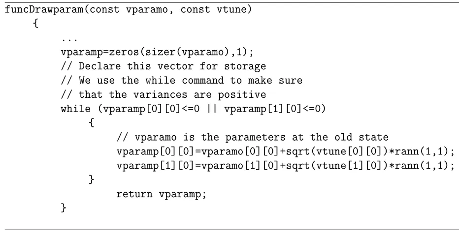
❢✉♥❝❉r❛✇♣❛r❛♠✭❝♦♥st ✈♣❛r❛♠♦✱ ❝♦♥st ✈t✉♥❡✮ ④

✳✳✳

✈♣❛r❛♠♣❂③❡r♦s✭s✐③❡r✭✈♣❛r❛♠♦✮✱✶✮❀ ✴✴ ❉❡❝❧❛r❡ t❤✐s ✈❡❝t♦r ❢♦r st♦r❛❣❡

✴✴ ❲❡ ✉s❡ t❤❡ ✇❤✐❧❡ ❝♦♠♠❛♥❞ t♦ ♠❛❦❡ s✉r❡ ✴✴ t❤❛t t❤❡ ✈❛r✐❛♥❝❡s ❛r❡ ♣♦s✐t✐✈❡

✇❤✐❧❡ ✭✈♣❛r❛♠♣❬✵❪❬✵❪❁❂✵ ⑤⑤ ✈♣❛r❛♠♣❬✶❪❬✵❪❁❂✵✮ ④

✴✴ ✈♣❛r❛♠♦ ✐s t❤❡ ♣❛r❛♠❡t❡rs ❛t t❤❡ ♦❧❞ st❛t❡

✈♣❛r❛♠♣❬✵❪❬✵❪❂✈♣❛r❛♠♦❬✵❪❬✵❪✰sqrt✭✈t✉♥❡❬✵❪❬✵❪✮✯r❛♥♥✭✶✱✶✮❀ ✈♣❛r❛♠♣❬✶❪❬✵❪❂✈♣❛r❛♠♦❬✶❪❬✵❪✰sqrt✭✈t✉♥❡❬✶❪❬✵❪✮✯r❛♥♥✭✶✱✶✮❀ ⑥

Table 5: Marginal likelihood computation using Gelfand-Dey method in Ox

❢✉♥❝●❉✭❝♦♥st ♠t❤❡t❛✱ ❝♦♥st ♠♣r✐♦r✱ ❝♦♥st ✈❧♦❣♣❞❢✱ ❝♦♥st ✐s✐♠✱ ❝♦♥st ❞❛❧♣❤❛✮ ④

✳✳✳

✴✴ ♠t❤❡t❛ ✐s ✐s✐♠①✷ ✈❡❝t♦r ♦❢ ♣❛r❛♠❡t❡rs ✴✴ ▼❛❦❡ t❤❡ ❧♦♦♣ ✐♥ ♦r❞❡r t♦ ❡✈❛❧✉❛t❡ t❤❡ ♣❞❢ ♠♣❞❢❂③❡r♦s✭✐s✐♠✱s✐③❡❝✭♠t❤❡t❛✮✮❀

❢♦r ✭❥❂✵❀ ❥❁✐s✐♠❀ ❥✰✰✮ ④

✴✴ ❈♦♠♣✉t❡ ♣❞❢ ❛t ❡❛❝❤ ❞r❛✇

♠♣❞❢❬❥❪❬✵❪❂❢✉♥❝■●♣❞❢①✭♠t❤❡t❛❬❥❪❬✵❪✱♠♣r✐♦r❬✵❪❬✵❪✱♠♣r✐♦r❬✵❪❬✶❪✮❀ ♠♣❞❢❬❥❪❬✶❪❂❢✉♥❝■●♣❞❢①✭♠t❤❡t❛❬❥❪❬✶❪✱♠♣r✐♦r❬✶❪❬✵❪✱♠♣r✐♦r❬✶❪❬✶❪✮❀ ⑥

✴✴ ❈❛❧❝✉❧❛t❡ ♠❡❛♥ ❛♥❞ ✈❛r✐❛♥❝❡ ♦❢ t❤❡ ❞r❛✇s ✈♠❡❛♥❂♠❡❛♥❝✭♠t❤❡t❛✮❀ ♠❝♦✈❂✈❛r✐❛♥❝❡✭♠t❤❡t❛✮❀ ✈tr✉♥❝❂③❡r♦s✭✐s✐♠✱✶✮❀

✴✴ ❈❛❧❝✉❧❛t❡ ❣ ✈❢❂③❡r♦s✭✐s✐♠✱✶✮❀ ❢♦r ✭✐❂✵❀ ✐❁✐s✐♠❀ ✐✰✰✮

④

✴✴ ❢✉♥❝▼❱◆♣❞❢① ✐s ♠✉❧t✐✈❛r✐❛t❡ ◆♦r♠❛❧ ❞❡♥s✐t② ✭❛❧r❡❛❞② ✐♥ ❧♦❣✮

✈tr✉♥❝❬✐❪❬✵❪❂

✭♠t❤❡t❛❬✐❪❬❪✲✈♠❡❛♥✮✯✐♥✈❡rt✭♠❝♦✈✮✯ ✭♠t❤❡t❛❬✐❪❬❪✲✈♠❡❛♥✮✬❀

✈❢❬✐❪❬✵❪❂❢✉♥❝▼❱◆♣❞❢①✭♠t❤❡t❛❬✐❪❬❪✱✈♠❡❛♥✱♠❝♦✈✮✲❧♦❣✭❞❛❧♣❤❛✮❀ ⑥

❞❝r✐t✐❝❛❧❂q✉❛♥❝❤✐✭❞❛❧♣❤❛✱s✐③❡❝✭♠t❤❡t❛✮✮❀ ✈tr✉♥❝✐❂✈tr✉♥❝❃❞❝r✐t✐❝❛❧❀

✴✴ ❙❡t t❤✐s t♦ ❜❛s✐❝❛❧❧② ③❡r♦ ✐❢ ✇❡ ✴✴ ❡①t❡♥❞ t❤❡ tr✉♥❝❛t✐♦♥ ❧✐♠✐t ✴✴ ✐✳❡ ❞✐s❝❛r❞ t❤❡s❡ ❞r❛✇s ✈❢❬✈tr✉♥❝✐❪❬❪❂✲✳■♥❢❀

✈❧♦❣●❉❂✈❢✲s✉♠r✭♠♣❞❢✮✲✈❧♦❣♣❞❢❀ ❞❝♦♥st❛♥t❂♠❛①✭✈❧♦❣●❉✮❀

✴✴ ❈❛❧❝✉❧❛t❡ ♠❛r❣✐♥❛❧ ❧✐❦❡❧✐❤♦♦❞

❞♠❧❂✲❞❝♦♥st❛♥t✲❧♦❣✭♠❡❛♥❝✭❡①♣✭✈❧♦❣●❉✲❞❝♦♥st❛♥t✮✮✮❀ r❡t✉r♥ ❞♠❧❀

Table 6: Estimation results of unobserved component (UC) models

UC UC-SVm UC-SV

Parameter θ¯ RB θ¯ RB θ¯ RB

µ1 0.0602 4.08 -0.0764 8.47

[-0.4104, 0.5197] [-0.3733,0.2223]

µ2 -0.5886 4.95

[-0.9465,-0.2391]

φ1 0.9456 4.54 0.9541 7.84

[0.9067,0.9792] [0.9278,0.9779]

φ2 0.9815 7.21

[0.9676,0.9938]

σ₁2 3.2280 5.09 0.1153 3.93 0.0844 8.97 [2.9026,3.5680] [0.0408,0.2215] [0.0383,0.1406]

σ2

2 2.0021 4.57 0.5090 3.59 0.0141 7.75

[1.2772,2.7866] [0.3449,0.6826] [0.0051,0.0255]

log(L) -592.28 -469.35 -465.07

log(ML),a=0.75 -638.30 -497.77 -484.86 log(ML),a=0.99 -638.03 -497.50 -484.58

M-H ratio 0.42 0.48 0.40

Table 7: Simulation evidence, ARFIMA-SV

ARFIMA(0,d,0)-SV ARFIMA(0,d,0)

Parameter true θ¯ RB θ¯ RB

τ 0.70 0.5783 6.19 2.0887 7.45 [0.0270,1.1633]

d 0.35 0.3301 5.36 0.3406 6.37 [0.2970,0.3623]

µ 1.20 1.4317 5.37 [1.1736,1.6831]

φ 0.97 0.9666 4.67 [0.9551,0.9781]

σ2 _{0.05 0.0523 5.26 6.0434 1.02}

[0.0361 ,0.0699]

log(L) -2203.3 -2321.9

log(ML),a=0.75 -2221.4 -2353.4 log(ML),a=0.99 -2221.1 -2354.1

M-H ratio 0.38

Table 8: Estimation results, ARFIMA-SV and ARFIMA

ARFIMA(0,d,0)-SV ARFIMA(1,d,0)-SV ARFIMA(0,d,0)

Parameter θ¯ RB θ¯ RB θ¯ RB

τ 0.1331 5.42 0.1086 5.80 0.2657 6.69

[0.0763,0.1886] [0.0324,0.1827] [0.1261,0.4009]

d 0.3509 6.22 0.4609 8.06 0.3968 4.44

[0.3206,0.3829] [0.4281,0.4926] [0.3491,0.4453]

ρ -0.2835 6.75

[-0.3335,-0.2328]

µ -3.5845 5.38 -3.4799 6.46

[-4.0077,-3.1675] [-3.9046,-3.0321]

φ 0.9871 5.74 0.9870 7.04

[0.9828,0.9898] [0.9831,0.9897]

σ2 _{0.0175 5.78 0.0191 6.61 0.0293 1.02}

[0.0108,0.0249] [0.0124,0.0267] [0.0263,0.0326]

log(L) 337.77 353.37 218.70

log(ML),a=0.75 315.00 327.08 209.25

log(ML),a=0.99 315.28 327.36 209.22

M-H ratio 0.39 0.39

This table reports estimation results for different ARFIMA(p,d,q)models using US core inflation rate data. log(L): loglikelihood, log(ML): log-marginal likelihood for the corresponding value of

a. M-H ratio: Metropolis-Hastings acceptance ratio.

Table 9: Out-of-sample forecast results,yt+h

MAE RMSE

Model h=1 h=4 h=8 h=1 h=4 h=8 AR(1) 0.1173 0.1633 0.1786 0.1656 0.2187 0.2350 AR(4) 0.1075 0.1296 0.1423 0.1552(∗) 0.1851 0.1889

ARMA(1,1) 0.1026 0.1185 0.1291 0.1500(∗) 0.1751 0.1771

ARFIMA(0,d,0) 0.1010(∗) 0.1167 0.1257 0.1480(∗) 0.1717 0.1787 ARFIMA(1,d,0) 0.1028 0.1154 0.1255 0.1491(∗) 0.1697 0.1766 ARFIMA(0,d,0)-SV 0.1002(∗) 0.1139 0.1205 0.1474(∗) 0.1695 0.1753 ARFIMA(1,d,0)-SV 0.1011(∗) 0.1105(∗) 0.1164(∗) 0.1479(∗) 0.1665(∗) 0.1707(∗)

Table 10: Simulation evidence

DGP: stochastic volatility with MA(1) errors, SV-MA(1) DGP: stochastic volatility in mean, SVM

SV SV-MA(1) SV SVM

Parameter true θ¯ RB θ¯ RB true θ¯ RB θ¯ RB

µ 0.20 0.4168 4.31 0.2756 4.40 0.20 0.7287 23.72 0.2883 5.24

[0.2129,0.6045] [0.0419,0.5011] [0.4106,1.0132] [0.0580,0.5191]

φ 0.98 0.9701 5.07 0.9781 4.55 0.98 0.9815 21.63 0.9790 4.86

[0.9515,0.9861] [0.9635,0.9906] [0.9651,0.9928] [0.9655,0.9904]

σ2 _{0.01 0.0171 4.86 0.0104 5.22 0.01 0.0087 0.0108 5.38}

[0.0078,0.0291] [0.0048,0.0172] [0.0043,0.0159] 14.04 [0.0055,0.0174]

ψ 0.40 0.4591 5.57

[0.4221,0.4963]

β 0.80 0.7533 5.09

[0.7090,0.8001]

log(L) -1666.1 -1581.0 -1811.0 -1586.8

log(ML),a=0.75 -1671.2 -1592.4 -1817.5 -1598.5

log(ML),a=0.99 -1673.8 -1592.2 -1817.2 -1598.2

M-H ratio 0.42 0.38 0.33 0.37

This table reports estimation results for SV-MA(1) and SVM using simulated data. log(L): loglikelihood, log(ML): log-marginal likeli-hood for the corresponding value ofa. M-H ratio: Metropolis-Hastings acceptance ratio.

Figure 1: Estimation results, SVL model on OMXC20 daily returns

OMXC20

2006 2008 2010 2012 200

400 600

OMXC20 Daily returns

2006 2008 2010 2012 −20

0 20

Daily returns E(σ_t|y₁,...,y_T)

20060 2008 2010 2012 2

4 6

E(σ_t|y₁,...,y_T)

Loglike (PF)

0 2500 5000 7500 10000 −2175

−2150 −2125 −2100

Loglike (PF)

µ|Y_T

0 2500 5000 7500 10000 −0.5

0.5 1.5 _µ

|Y_T

φ|Y_T

0 2500 5000 7500 10000 0.90

0.95 1.00

φ|Y_T

σ2_|Y

T

0 2500 5000 7500 10000 0.00

0.04

0.08 _σ2_|Y

T ρ|YT

0 2500 5000 7500 10000 −0.5

0.0 0.5 _ρ

|Y_T

µ|Y_T

−0.50 0.5 1.5 1

2 3 _µ|

Y_T φ|Y_T

0.900 0.95 1.00 50

100 150 _φ

|Y_T σ2|Y_T

0.00 0.04 0.08 25

50

75 _σ2_|Y

T ρ|YT

−0.5 0.0 0.5

2.5 5.0 7.5 _ρ

|Y_T

µ

0 100 200 300 400 500 −1

0

1 _{µ φ}

0 100 200 300 400 500 −1

0

1 _{φ σ2}

0 100 200 300 400 500 −1

0 1 _σ2

ρ

0 100 200 300 400 500 −1

0

1 _ρ

Figure 2: Estimation results, UC-SV

Inflation Filtered trend

1952 1962 1972 1982 1992 2002 2012 −16

−6 4 14 24

Inflation Filtered trend 1st difference of inflation

1952 1962 1972 1982 1992 2002 2012 −16

−6 4 14 24

1st difference of inflation

Irregular volatility

19520 1962 1972 1982 1992 2002 2012 2

4 6 8

Irregular volatility Regular volatility

1952 1962 1972 1982 1992 2002 2012 0.0

0.4 0.8 1.2 1.6

Regular volatility

Figure 3: Estimation results, ARFIMA(1,d,0)-SV

US core inflation

1960 1970 1980 1990 2000 2010 −0.5

0.0 0.5 1.0 1.5

US core inflation exp(α_t/2)

1960 1970 1980 1990 2000 2010 0.0

0.1 0.2 0.3 0.4

exp(α_t/2)

d|Y_T

0 2000 4000 6000 8000 10000 0.40

0.45 0.50 0.55

d|Y_T ρ|Y_T

0 2000 4000 6000 8000 10000 −0.4

−0.3 −0.2 −0.1

ρ|Y_T

d

0 100 200 300 400 500

−1 0 1

d ρ

0 100 200 300 400 500

−1 0 1

ρ

Figure 4: Rolling window parameter estimates, ARFIMA(1,d,0)-SV

1960 1965 1970 1975 1980 1985 1990 1995 0.0

0.2 0.4 0.6 0.8

(a)

1960 1965 1970 1975 1980 1985 1990 1995 0.1

0.2 0.3 0.4 0.5

(b)

1960 1965 1970 1975 1980 1985 1990 1995 −0.45

−0.30 −0.15 0.00 0.15

(c)

1960 1965 1970 1975 1980 1985 1990 1995 0.0

0.3 0.6 0.9 1.2

(d)