Fuzzy integral driven ensemble classification using a priori fuzzy measures

Fuzzy Integral Driven Ensemble Classification using

A Priori Fuzzy Measures

Utkarsh Agrawal

, Christian Wagner

, Jonathan M. Garibaldi

, Daniele Soria

Lab for Uncertainty in Data and Decision Making (LUCID), School of Computer Science,University of Nottingham, Nottingham, UK 2. School of Computer Science and Engineering, University of Westminster,London, UK email:{utkarsh.agrawal, christian.wagner, jon.garibaldi}@nottingham.ac.uk, [email protected]

Abstract—Aggregation operators are mathematical functions that enable the fusion of information from multiple sources. Fuzzy Integrals (FIs) are widely used aggregation operators, which combine information in respect to a Fuzzy Measure (FM) which captures the worth of both the individual sources and all their possible combinations. However, FIs suffer from the potential drawback of not fusing information according to the intuitively interpretable FM, leading to non-intuitive results. The latter is particularly relevant when a FM has been defined using external information (e.g. experts). In order to address this and provide an alternative to the FI, the Recursive Average (RAV) aggregation operator was recently proposed which enables intuitive data fusion in respect to a given FM. With an alternative fusion operator in place, in this paper, we define the concept of ‘A Priori’ FMs which are generated based on external information (e.g. classification accuracy) and thus provide an alternative to the traditional approaches of learning or manually specifying FMs. We proceed to develop one specific instance of such an a prioriFM to support the decision level fusion step in ensemble classification. We evaluate the resulting approach by contrasting the performance of the ensemble classifiers for different FMs, including the recently introduced Uriz and the Sugeno λ -measure; as well as by employing both the Choquet FI and the RAV as possible fusion operators. Results are presented for 20 datasets from machine learning repositories and contextualised to the wider literature by comparing them to state-of-the-art ensemble classifiers such as Adaboost, Bagging, Random Forest and Majority Voting.

I. INTRODUCTION

Aggregation operators are powerful mathematical methods for weighted multi-source information fusion. The weights of the sources (e.g. individual classifier outputs in the context of ensemble classification) are defined by a Fuzzy Measure (FM) [1], [2], which captures the worth of the individual sources and all their possible combinations. Many aggregation operators have been proposed in the literature, Fuzzy Integrals (FIs) [3] being the most commonly used (especially the Choquet Fuzzy Integral (CFI)).

Although FIs have been used widely, they suffer from po-tential drawbacks of producing non-intuitive results in respect to a commonly intuitively interpretable FM. For example, as shown in [4], the re-ordering inherent to the FI can lead to only partial exploitation of a FM and the aggregation of symmetrically mirrored inputs does not necessarily result in symmetrically mirrored outputs. Wagner et al. recently

discussed these aspects in detail in [4] and introduced a family of aggregation functions called the Recursive Average (RAV), as an alternative to FIs for fusion applications designed to leverage (interpretable) FMs. With the RAV operator address-ing some of the potential shortcomaddress-ings of how FMs are used by FIs, there is renewed scope to revisit how FMs are generated in practical applications.

Currently, to construct a FM, three key approaches are common: 1) Expert-driven, 2) Algorithm-driven and 3) Op-timisation (see Section II-A). In this paper, we put forward a fourth category: FMs specified using externally available information, so-called a priori FMs. The key idea underpin-ning these FMs is that they are specified independently of the actual aggregation operator using external information, thus preserving their interpretability. Here, ‘external information’ is information available to inform the weighting of individual sources and their combinations which is independent from the actual data fusion step. In this sense, one could argue that expert-driven FMs are also a type of ‘a priori’ FM; nevertheless, as expert-driven FMs are a specific type with a long and well understood tradition/rationale, we argue that maintaining them as a separate category is both useful and serves clarity.

In the context of ensemble classification, the aggregation operators are an extension of the weighted ensemble al-gorithms. In the past decade, aggregation operators based ensemble classifiers have become popular due to their ability to express interactions between the classifiers [5], [6]. In this paper, we develop one specific instance of an a priori FM: one which captures the quality of individual classifiers (and their combinations) in order to then enable a fusion-based ensemble classifier. While working on this paper, the authors became aware of recent work by Uriz et al. [7] which introduces a FM based on the same principle (i.e. a FM based on sub-classifier performance) in the context of imbalanced classification problems and traditional FIs.

RAV operators, we focus only on the arithmetic RAV (i.e.

p = 1) in this paper. Experiments are conducted using 20 datasets from machine learning repositories and contextualised to the wider literature by comparing them to state-of-the-art ensemble classifiers such as Adaboost, Bagging, Random Forest and Majority Voting.

In Section 2 we review the background on FMs, Aggrega-tion operators and ensemble classificaAggrega-tion methods employed in this paper. In Section 3 the a priori FM is introduced. This section also presents the a priori FM based ensemble classifier. Section 4 presents and discusses the results of all the experiments, followed by conclusion in Section 5.

II. BACKGROUND

A. Fuzzy Measures

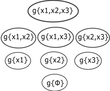
Fuzzy Measures (FMs) capture the worth of each infor-mation source (also called densities) and all their possible combinations i.e. every subset in a power set [1], [4]. Figure 1 shows the FM weight structure (also referred as a lattice) for three sources.

Let X = {x1, ..., xn} be a discrete and finite set of

information sources and g : 2X _{→ [0,1] be a FM having}

the following properties:

P1: Boundary condition, i.e.,g(∅) = 0, g(X) = 1, and P2: Monotonic and non-decreasing, i.e., g(A) ≤g(B) ≤1,

if A⊆B⊆X.

In cases of infinite FM X, there is another property which guarantees continuity. However, X is finite and discrete in this paper and therefore this property is not relevant. In the context of ensemble classification,g(A)represents the weight or importance of subset A. To construct FMs there are three major approaches, as follows:

1) Expert-driven:While FMs can be defined by experts [4], with increasing lattice size (number of parameters), defining each parameter of the FM becomes practically not feasible, restricting this approach to a subset of applications with a limited number of sources.

2) Algorithm-driven:These methods compute the FM from the values of individual sources by leveraging the FM’s mathematical constraints. Some examples are the Sugenoλ-measure, the S-decomposable measure and the K-additive measure [8]–[11].

3) Optimisation-driven: These methods use algorithms such as gradient descent, evolutionary computation and quadratic programming to optimise the FMsin respect to a pre-defined aggregation operatorand training data [1], [5], [12]. Note that this approach, while offering the potential of powerful and concise fusion operators, is also most at risk of generating non-generic FMs, i.e. FMs which are not independently interpretable, but are tuned to drive the specific aggregation operator (e.g. CFI) which they were trained for [4].

One of the extensively used FM in a number of research works is the Sugeno λ-measure, described in the next sub-section.

Fig. 1: FM Lattice for three sources

1) Sugeno λ-measure: Introduced by Sugeno [13], the Sugeno λ-measure has been the most commonly used algo-rithmic FM in literature.

The Sugenoλ-measure centres on the following property:

P3: ∀ A, B∈X,A∩B=φ,

g(A∪B) =g(A) +g(B) +λg(A)g(B),

where λ > −1. The unique value of λ can be obtained by solving the following polynomial equation:

1 +λ=

n

Y

i=1

(1 +λgi),

wheregi=g(xi).

2) Uriz FM: Uriz et al. [7] proposed a method which learns the FM from the classification accuracies of individual classifiers. This method shares key aspects of the motivation in respect to using the performance of individual classifiers within an ensemble classification framework with the approach put forward in this paper, nevertheless follows a different approach in the generation of the actual FM as detailed in Section III.

For all A ⊆ X and a number of classifiers (or features)

N : {1, .., n}, the Uriz’s FM is composed in two steps. First, the uniform FM gu is given by:

gu(A) =

|A| n ,

The second step makes use of the results of all the individual classifiers and the results of all classifier combinations, given byAccA,∀A⊆X, as follows:

g(A) =gu(A) +

tanh(AccA−M eanAcc|A|)

2n ,

B. Aggregation Operators

Aggregation operators are mathematical functions that com-bine the information from multiple sources [1], [4]. There are many aggregation operators in the literature [14], but in this work we focus on commonly used FIs and the recently introduced RAV, explained in the next subsections.

1) Fuzzy Integrals: Fuzzy Integrals (FIs) are non-linear aggregation functions often used for information (evidence) fusion using the worth of each subset of sources (provided by a FM ‘g’) [1], [4]. The two most commonly used FIs in the literature include Choquet Fuzzy Integral (CFI) [1], [2], [5], [6] and Sugeno Fuzzy Integral (SFI) [3]. In this work the CFI is used which is defined as follows:

Choquet Fuzzy Integral: Let h : X → [0,∞) be a real valued function that represents the evidence or support of a hypothesis. The discrete Choquet Fuzzy Integral (CFI) [1]–[4] can be defined as:

Z

CF I

h◦g=CF Ig(h) = n

X

i=1

h(xπ(i))[g(Ai)−g(Ai−1)] (1) where π is a permutation of X such that h(xπ(1)) ≥ h(xπ(2)) ≥ ... ≥ h(xπ(n)), Ai = [xπ(1), ..., xπ(n)] and g(A0) = 0. More detail on the property of FIs and the CFI can be found in [14].

2) Recursive Average (RAV): The Recursive Average (RAV), an instance of Recursive Weighted Power Mean − introduced by Wagner et al. [4], is an aggregation operator that fuses information over a set of sources X defined with respect to a FM g, mathematically defined as follows:

RAVp(X) =

(

h(X), if|X|= 1.

(Pg(Bj)∗RAVp(Bj)p

P_g(B

j)

1/p

, otherwise. (2)

where|p|>0, Bj =X\xj, xj∈X.

∀pthe RAV for a set of sources is recursively defined as the weighted average of its sub sources, where the weight at each node is captured by a FM [4]. For some particular p

values, RAV adopts specific averaging behaviour in a recursive manner, i.e. the recursive arithmetic average for p = 1, the recursive harmonic average forp=−1, the recursive quadratic average for p= 2, and so on. For simplicity and space, we focus on solely on the RAV forp= 1in this paper.

C. Ensemble Classification

Ensemble Classification determines the class to which a new object belongs by integrating the results of multiple classifiers. In the previous studies [1], [6], [15], the researchers concluded that aggregation operator based ensemble classifiers worked well in a number of applications such as multi-criteria decision making (MCDM) [16], forensic science [17], software defect prediction [18], brain computer interface (BCI) [19], computer vision [20], [21] and explosive hazard detection [22]. Here, we use the application of ensemble classification to compare the a priori measure with the Sugeno λ-measure and the Uriz measure.

Algorithm 1: a prioriFM Algorithm

inputs :Accuracy Values (Acc), normalisation factor (Nf)

output:Fuzzy Measure (gap)

M axAcc= arg max(Acc)

foreach iinnm(A)do

S1:

nm(Ai) = 1−

M axAcc−Acc(i)

M axAcc−Nf

S2:

if|A|== 1then gap(Ai) =nm(Ai);

else

ifnm(Ai)< nm(Bi)then

gap(Ai) =nm(Bi);

else

gap(Ai) =nm(Ai);

where,nm(Bi) =max(gap(A−1i))

Importantly, the FM based ensemble classifiers are also compared with extensively used, state-of-the-art, machine learning algorithms methods such as the Random Forests, Bagging, Boosting and Majority Voting (briefly explained below). Finally, We also compare the a priorimeasure based classifier with DeFIMKL [5] (Decision-level Fuzzy Integral Multiple Kernel Learning), which is a state-of-the-art FI based ensemble classification algorithm.

Adaboost: Adaboost is a very popular ensemble classifi-cation algorithm which combines multiple weak classifiers to construct a strong classifier [23]. The algorithm trains by giving higher weights to mis-classified data in subsequent iteration (of the classifier) while the weights of the correctly classified instances are decreased. Weighted combinations of all the classifiers in the ensemble are used to predict the final result.

Bagging: Bagging (or Bootstrap Aggregation) [24] ensem-ble algorithms are most commonly used in proensem-blems with high variance. The data for each classifier in the ensemble is selected by sampling with replacement. The final classification outcome is based on a majority-vote.

Majority Voting with SVM (MJSVM): Letxbe an instance and Si (i = 1,2, ..., k) Support Vector Machine (SVM)

classifiers that output class labels mi(x, cj). For each class

label cj (where j = 1, ..., n) [15], the output of the final

classifiery(x)for instancexis given by:

y(x) = maxcj

k

X

i=1

mi(x, cj). (3)

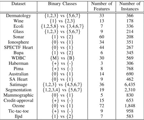
TABLE I: Dataset Description

Dataset Binary Classes Number of Number of

Features Instances

Dermatology {1,2,3}vs{5,6,7} 33 366

Wine {1}vs{2,3} 13 178

Ecoli {1,2,5,8}vs{3,4,6,7} 7 336

Glass {1,2,3}vs{5,6,7} 9 214

Sonar {1}vs{2} 60 208

Ionosphere {0}vs{1} 34 351

SPECTF Heart {0}vs{1} 44 267

Bupa {1}vs{2} 6 345

WDBC {M}vs{B} 30 569

Haberman {+}vs{-} 3 306

Pima {+}vs{-} 8 768

Australian {0}vs{1} 14 690

SA Heart {0}vs{1} 9 462

Satimage {1,2,3}vs{4,5,6,7} 36 6,435

Segmentation {1,2,3,4}vs{5,6,7} 19 2,310

Mammographic {0}vs{1} 5 830

Credit-approval {+}vs{-} 15 653

Ozone {0}vs{1} 72 1,848

Tic-tac-toe {+}vs{-} 9 958

Ilpd {1}vs{2} 7 583

DeFIMKL algorithm: The Decision-level Fuzzy Integral

MultipleKernelLearning (DeFIMKL) is a state-of-the-art FI-FM ensemble classification algorithm, which aggregates the kernels through the use of the CFI with respect to a FM learned by a regularised quadratic programming approach [1]. Agrawal et al. [15] showed that DeFIMKL is the best FI-FM ensemble classification algorithm, therefore it will be informative to compare DeFIMKL with the a priori FM based ensemble classifier.

III. A PrioriFMFORENSEMBLECLASSIFICATION

This section presents an instance of anA priori FM which uses the classification accuracy of all the individual classifiers and their combinations as external information. The steps of the algorithm using thea prioriFM for ensemble classification is also presented in this section.

A. Generating an A priori FM for Ensemble Classification

For all the classifier combinationsA⊆X and the classifiers in the ensemble N : {1, .., n}, the a priori FM is given by ‘gap’, presented in Algorithm 1. Algorithm 1 takes as input the

classification accuracies Acci (i.e. the training set accuracies

of the input dataset), whereiis all the combinations, and the normalisation factorNf(the range on which the accuracies are

normalised); and generates thea prioriFMgapby running the

following steps:

S1: The input accuracies are normalised using the factor

Nf = 50i.e. the input accuracies are normalised between

50% and the maximum observed accuracy (M axAcc). The normalisation factor is chosen to be 50 (instead of 0) as the classifiers should ideally perform better than random guessing i.e. their accuracies should be more than 50%. These normalised accuracies are then subtracted from one (to give high worth to best accuracies and vice-versa) and then passed on to second step.

S2: For all the individual classifiers (eg g{x1}, g{x2} and g{x3}from Fig. 1), the values obtained from the previous step is the final a priori FM value. For each combina-tion of sources (eg all the combinacombina-tions in Fig 1), if the normalised measure value obtained from the previ-ous step is greater than or equal to the values of all its sub-sources, the normalised measure value of that combination is the final a priori FM (eg from Fig 1 if nm({x1, x2}) > nm({x1}) and nm({x1, x2}) > nm({x2}), then gap({x1, x2}) = nm({x1, x2})) . Otherwise, if this normalised measure value is less than the measure value of any of its sub-sources, the maximum measure value among its sub-sources is the final a priori FM (eg from Fig 1 if nm({x1, x2}) < nm({x1}) or nm({x1, x2})< nm({x2})or both, then gap({x1, x2}) = max(nm({x1}), nm({x2}))). B. Ensemble Classification

Each test datax0can be classified using the following steps: 1) Compute the decision value h(x0)for all the classifiers

in the ensemble,

2) The aggregation valueaggfor the test data is computed using thea prioriFMgapin respect to the RAV (2) or

the CFI (1).

3) The final class label issign(agg).

IV. RESULTS ANDDISCUSSION

In this section we present the experimental framework for the comparison of the FM based ensemble classifiers followed by results and discussion.

A. Experimental Framework

The a priori FM is compared with Uriz and Sugeno FMs, for both the RAV and the CFI aggregation operators, for 20 benchmark datasets from the UCI machine learning repository [26], described in Table I. To be consistent, the comparison with the DeFIMKL, MJSVM, Adaboost (with trees), Bagging and Random Forest ensemble classifiers is also presented for the same 20 datasets. All these datasets are normalised using zero mean and unit standard-deviation normalisation [27]. A binary ensemble classifier is used for comparison. As many of the datasets have more than two classes, classes are merged in the datasets having more than two classes [28].

B. Results

TABLE II:Summary performance statistics of theA prioriFM, the Uriz FM and the Sugenoλ-measure based ensemble classifiers for the same base classifiers. For clarity, the best classifiers are bold, the classifiers performances which are statistically significantly indifferent

than the best are initalicsand the ones which are statistically significantly worse than the best are underlined.

Datasets Sugeno Sugeno Uriz Uriz A priori A priori

CFI RAV CFI RAV CFI RAV

Dermatology 96.85 (2.07) 97.14 (1.98) 97.16 (1.94) 97.18 (1.94) 96.81 (2.16) 97.15 (1.97) Wine 98.86 (2) 99.16 (1.66) 99.16 (1.66) 99.16 (1.66) 98.86 (2) 99.16 (1.66)

Ecoli 96.87 (2.08) 96.71 (2.13) 96.68 (2.13) 96.68 (2.13) 96.88 (2.1) 96.71 (2.13) Glass 92.91 (3.95) 92.43 (4.32) 92.41 (4.3) 92.34 (4.34) 92.93 (3.95) 92.43 (4.32) Sonar 80.42 (6.1) 80.35 (6.33) 80.53 (6.4) 80.56 (6.21) 80.51 (5.99) 80.44 (6.34) Ionosphere 94.68 (2.65) 94.1 (2.59) 94.13 (2.63) 94.13 (2.63) 94.69 (2.66) 94.13 (2.61) SPECTF Heart 80.13 (5.23) 80.09 (5.2) 80.02 (5.09) 80 (5.08) 80.11 (5.19) 80.06 (5.19) Bupa 67.35 (5.16) 67.74 (5.39) 67.75 (5.37) 67.65 (5.27) 67.36 (5.23) 67.75 (5.34)

WDBC 96.72 (1.79) 96.83 (1.79) 96.83 (1.78) 96.83 (1.83) 96.7 (1.79) 96.83 (1.78)

Haberman 73.03 (4.7) 73.19 (4.8) 73.19 (4.8) 73.21 (4.83) 73.05 (4.68) 73.21 (4.81)

Pima 75.94 (2.86) 75.95 (2.82) 75.95 (2.82) 75.97 (2.84) 75.95 (2.99) 75.95 (2.83) Australian 84.86 (3.03) 85.13 (2.93) 85.14 (2.96) 85.13 (2.92) 84.75 (3.01) 85.14 (2.94)

SA Heart 70.99 (4.11) 71.13 (4.13) 71.13 (4.11) 71.18 (4.13) 70.95 (4.08) 71.13 (4.13) Satimage 95.29 (0.53) 95.22 (0.55) 95.22 (0.55) 95.23 (0.55) 95.28 (0.53) 95.22 (0.55) Segmentation 91.17 (1.21) 91.66 (1.17) 91.71 (1.16) 91.76 (1.17) 91.17 (1.22) 91.67 (1.17) Mammographic 82.38 (3.37) 82.36 (3.67) 82.37 (3.69) 82.37 (3.69) 82.42 (3.39) 82.37 (3.66) Credit-approval 86.29 (2.38) 86.52 (2.41) 86.49 (2.41) 86.5 (2.4) 86.28 (2.38) 86.52 (2.41)

Ozone 96.87 (0.79) 96.87 (0.79) 96.87 (0.79) 96.87 (0.79) 96.87 (0.79) 96.87 (0.79)

Tic-tac-toe 86.23 (2.29) 84.97 (2.67) 85.09 (2.62) 85.28 (2.56) 86.33 (2.34) 85.01 (2.64) Ilpd 70.95 (3.31) 71.07 (3.44) 71.08 (3.44) 71.08 (3.44) 70.91 (3.28) 71.08 (3.44)

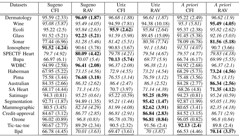
TABLE III: Summary performance statistics of theA prioriFM, the Uriz FM and the Sugenoλ-measure based ensemble classifiers with mixed classifiers. For clarity, the best classifiers are bold, the classifiers performances which are statistically significantly indifferent than

the best are initalicsand the ones which are statistically significantly worse than the best are underlined.

Datasets Sugeno Sugeno Uriz Uriz A priori A priori

CFI RAV CFI RAV CFI RAV

Dermatology 95.59 (2.33) 96.69 (1.87) 96.68 (1.88) 96.61 (1.87) 95.22 (2.49) 96.62 (1.9) Wine 95.08 (5.87) 95.49 (4.05) 94.59 (7.81) 94.38 (10.18) 95.3 (5.81) 95.49 (4.05)

Ecoli 95.22 (2.5) 95.84 (2.63) 95.9 (2.62) 95.84 (2.64) 95.37 (2.38) 95.82 (2.62) Glass 91.52 (5.21) 92.23 (5.21) 91.59 (5.98) 89.45 (15.09) 91.45 (5.38) 92.16 (5.03) Sonar 77.44 (6.96) 81.28 (5.46) 81.42 (5.51) 80.56 (7.74) 78.09 (6.78) 81.56 (5.18)

Ionosphere 91.52 (4.24) 90.61 (3.78) 90.83 (3.67) 91.1 (3.84) 91.51 (4.07) 90.7 (3.66) SPECTF Heart 79.7 (4.92) 80.09 (4.42) 79.78 (4.21) 79.54 (4.67) 79.57 (4.77) 79.83 (4.18)

Bupa 66.97 (6.1) 70.07 (5.4) 70.13 (5.74) 69.77 (5.9) 66.74 (6.17) 69.99 (5.55) WDBC 94.99 (2.58) 96.41 (2.08) 96.37 (2.08) 96.38 (2.1) 94.92 (2.68) 96.37 (2.1) Haberman 67.95 (5.22) 73.15 (4.56) 72.9 (4.55) 73.21 (4.54) 68.29 (5.73) 73.24 (4.56)

Pima 75.58 (3.44) 76.68 (3.18) 76.55 (3.14) 76.59 (3.12) 75.48 (3.56) 76.5 (3.15) Australian 84.35 (2.66) 86.32 (2.62) 86.4 (2.47) 86.3 (2.52) 84.28 (2.77) 86.34 (2.56)

SA Heart 68.17 (4.44) 71.3 (4.15) 70.7 (3.97) 71.14 (4.38) 68.26 (4.8) 71.35 (4.12)

Satimage 94.3 (0.81) 95.25 (0.61) 95.22 (0.59) 95.25 (0.59) 94.23 (0.81) 95.24 (0.59) Segmentation 92.71 (1.87) 94.89 (1.35) 95.21 (1.44) 95.42 (1.47) 92.87 (1.99) 95.05 (1.39) Mammographic 80.5 (3.45) 82.14 (4.29) 81.99 (4.08) 82.62 (3.91) 80.65 (3.41) 82.35 (4.18) Credit-approval 84.67 (3.12) 86.77 (2.85) 86.81 (2.91) 86.84 (2.83) 84.52 (3.15) 86.71 (2.9)

Ozone 96.02 (0.89) 96.8 (0.83) 96.78 (0.78) 96.81 (0.84) 96.05 (0.82) 96.8 (0.84) Tic-tac-toe 90.67 (2.77) 89.29 (2.34) 90.5 (2.32) 91.56 (2.4) 92.13 (2.4) 89.8 (2.4)

Ilpd 66.78 (4.45) 70.01 (3.63) 69.47 (3.61) 70 (3.87) 66.53 (4.46) 70.14 (3.57)

five different base classifiers i.e. SVM, Decision Tree, Ad-aboost, Bagging and Neural Network. Thea priori FM based aggregation operators (both CFI and RAV) performed best across the five SVM base classifiers and thus are compared against state-of-the-art ensemble classification algorithms: De-FIMKL, MJSVM, Adaboost with trees, Bagging and Random Forest, as reported in Table IV.

All the tables report the average and the standard-deviation accuracies for 100 runs of these runs. During each run 80% of

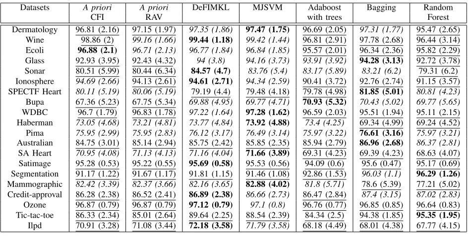
TABLE IV: Summary performance statistics of theA priori FM based ensemble classifier comparison with state-of-the-art ensemble classifiers. For clarity, the best classifiers are bold, the classifiers performances which are statistically significantly

indifferent than the best are initalicsand the ones which are statistically significantly worse than the best are underlined.

Datasets A priori A priori DeFIMKL MJSVM Adaboost Bagging Random

CFI RAV with trees Forest

Dermatology 96.81 (2.16) 97.15 (1.97) 97.35 (1.86) 97.47 (1.75) 96.69 (2.05) 97.31 (1.77) 95.47 (2.65) Wine 98.86 (2) 99.16 (1.66) 99.44 (1.18) 99.42 (1.44) 96.81 (2.91) 97.78 (2.68) 96.44 (3.14) Ecoli 96.88 (2.1) 96.71 (2.13) 96.77 (1.84) 96.84 (1.85) 95.57 (2.01) 96.34 (2.36) 95.82 (2.29) Glass 92.93 (3.95) 92.43 (4.32) 94 (3.8) 94.16 (3.73) 93.91 (3.92) 94.28 (3.13) 92.72 (3.78) Sonar 80.51 (5.99) 80.44 (6.34) 84.57 (4.7) 83.76 (5.4) 83.17 (5.89) 83.21 (6.2) 79.31 (6.2) Ionosphere 94.69 (2.66) 94.13 (2.61) 94.61 (2.71) 94.34 (2.59) 90.41 (3.72) 92.76 (2.74) 91.15 (3.57) SPECTF Heart 80.11 (5.19) 80.06 (5.19) 79.19 (4.4) 79.48 (4.18) 79.78 (4.98) 81.85 (5.01) 80.81 (4.23) Bupa 67.36 (5.23) 67.75 (5.34) 69.88 (4.95) 69.77 (4.71) 70.93 (5.32) 70.43 (5.02) 69.77 (5.65) WDBC 96.7 (1.79) 96.83 (1.78) 97.22 (1.64) 97.28 (1.62) 96.59 (2.03) 95.51 (1.94) 95.11 (2.15) Haberman 73.05 (4.68) 73.21 (4.81) 73.77 (4.84) 73.92 (4.88) 73.4 (4.25) 69.34 (4.99) 69.24 (4.52) Pima 75.95 (2.99) 75.95 (2.83) 76.12 (3.17) 76.49 (3.14) 75.97 (3.22) 76.61 (3.16) 75.97 (3.21) Australian 84.75 (3.01) 85.14 (2.94) 85.75 (2.42) 85.85 (2.35) 85.94 (2.79) 86.96 (2.68) 86.37 (2.81) SA Heart 70.95 (4.08) 71.13 (4.13) 71.16 (4.04) 71.66 (3.89) 69.31 (4.23) 69.39 (4.23) 68.63 (4.07) Satimage 95.28 (0.53) 95.22 (0.55) 95.69 (0.58) 95.53 (0.56) 94.09 (0.6) 95.6 (0.47) 95.17 (0.69) Segmentation 91.17 (1.22) 91.67 (1.17) 91.81 (1.15) 91.46 (1.08) 92.86 (1.53) 96.03 (1.1) 96.29 (1.26)

Mammographic 82.42 (3.39) 82.37 (3.66) 82.16 (3.65) 82.88 (4.02) 81.8 (5.71) 78.6 (5.39) 77.21 (5.02) Credit-approval 86.28 (2.38) 86.52 (2.41) 86.89 (2.38) 86.66 (2.73) 86.47 (2.84) 87.4 (3.15) 87.02 (2.83) Ozone 96.87 (0.79) 96.87 (0.79) 97.12 (0.79) 97.1 (0.8) 96.76 (0.77) 96.85 (0.85) 96.64 (0.83) Tic-tac-toe 86.33 (2.34) 85.01 (2.64) 89.64 (2.25) 88.54 (2.39) 84.34 (2.5) 94.38 (1.85) 95.35 (1.95)

Ilpd 70.91 (3.28) 71.08 (3.44) 72.18 (3.58) 71.79 (3.58) 68.18 (4.49) 68.01 (4.38) 67.77 (4.15)

C. Discussion

From Table II it can be observed that all the ensemble algorithms with the same base classifiers performed very well. Indeed, as shown in the table, nearly all classifiers result in performance which is not statistically different from the best classifier (hence nearly all results are shown in italics). In the below, we refer to best performance of a classifier when said classifier produces results which are either the best or statistically not different from the best.

The CFI based ensemble classifiers performed very simi-larly for all three measures, beingbestin 16 out of 20 datasets. The RAV operator based ensemble algorithm also performed very similarly, being best among 15 datasets for the Sugeno and theA priorimeasure, and 16 datasets for the Uriz measure. Overall, these algorithms outperformed all ensemble algo-rithms based on different base classifiers shown in Table III. Here, CFI based ensemble classifiers werebestin 2, 14 and 2 datasets for Sugeno, Uriz and A priori measure respectively. Conversely, RAV based ensemble algorithms were bestin 16, 15 and 17 datasets for Sugeno, Uriz and A priori measures respectively.

From Table IV it can be observed that the DeFIMKL and MJSVM were the overall best classifiers, showing good performance in 16 and 15 datasets respectively. The other classifiers: CFI with a priori FM, RAV with a priori FM, Adaboost with trees, Bagging and the Random Forest had the best accuracies in 7, 7, 6, 9 and 7 datasets respectively. DeFIMKL is the overall best FI based ensemble classifier, showing the performance of optimising the FM in respect to a specific operator (the CFI in this case). The a priori FM based classifiers (Which do not employ optimisation

towards a specific aggregation operator) overall achieve lower performance.

V. CONCLUSIONS

FIs are powerful aggregation operators, yet they suffer from potential drawbacks [4], resulting in non-intuitive outcomes when employed in respect to interpretable FMs, i.e. FMs which can be interpreted to provide meaningful insight into the value of information sources and their combinations.

The RAV aggregation operator was introduced as an alterna-tive to FIs, specifically for cases where a FM is available which is independent from the aggregation operator, for example a FM which is specified using external information (cf. experts). In this paper we put forward a new category ofa prioriFMs to capture FMs which are based on external information rather than for example being optimised in respect to training data and one specific aggregation operator such as the CFI.

The results show that the specific instance of an a priori FM put forward in this paper is a robust way to construct FMs which perform well (with different aggregation operators) in the context of ensemble classification. Results highlight the strong value of leveraging available information, rather than relying on FM generation approaches which focus solely on the densities (such as the Sugenoλ-measure) and the potential of alternative FM generation approaches which do not rely on training the FM in respect to one specific aggregation operator. In the future, we will focus on exploring the robustness of a priori FMs when employed with a wider set of aggregation operators, targeting the Sugeno FI as well as the CFI, but also the RAV operator for different values of p. Further, as part of an expanded journal paper on a priori FMs, we have developed a priori FMs which leverage external information from the scientific literature (and not the performance of individual classifiers as done in this paper) to support improved fusion, showing a pathway for delivering strong information aggregation using interpretable and validatable FMs, with rich scope for further research.

VI. ACKNOWLEDGEMENTS

The research was supported by The University of Notting-ham Vice-Chancellor’s Scholarship for Research Excellence (International).

REFERENCES

[1] A. J. Pinar, J. Rice, L. Hu, D. T. Anderson, and T. C. Havens, “Efficient Multiple Kernel Classification using Feature and Decision Level Fusion,” inIEEE Transactions on Fuzzy Systems, vol. 6706, no. c, 2016, pp. 1–1. [2] D. T. Anderson, S. R. Price, and T. C. Havens, “Regularization-based learning of the Choquet integral,” inIEEE International Conference on Fuzzy Systems, 2014, pp. 2519–2526.

[3] T. Murofushi and M. Sugeno, “A learning model using fuzzy measures and the Choquet integral,”Proc. of the 5th Fuzzy System Symposium, vol. 29, pp. 213–218, 1989.

[4] C. Wagner, T. C. Havens, and D. T. Anderson, “The Arithmetic Recursive Average as an Instance of the Recursive Weighted Power Mean,” inIEEE International on Conference Fuzzy Systems, 2017. [5] A. J. Pinar, T. C. Havens, M. A. Islam, and D. T. Anderson,

“Visual-ization and learning of the Choquet integral with limited training data,”

IEEE International Conference on Fuzzy Systems, 2017.

[6] Lequn Hu, D. T. Anderson, and T. C. Havens, “Multiple kernel aggre-gation using fuzzy integrals,”IEEE International Conference on Fuzzy Systems, 2013.

[7] M. Uriz, D. Paternain, H. Bustince, and M. Galar, “A first approach towards the usage of classifiers performance to create fuzzy measures for ensembles of classifiers: a case study on highly imbalanced datasets,” inIEEE International Conference on Fuzzy Systems, 2018.

[8] K. Fakhar, M. El Aroussi, M. N. Saidi, and D. Aboutajdine, “Apply-ing the upper integral to the biometric score fusion problem in the identification model,”IEEE International Conference on Electrical and Information Technologies (ICEIT), vol. 6, no. 3, pp. 494–504, 2015.

[9] Q. Wang, C. Zheng, H. Yu, and D. Deng, “Integration of heterogeneous classifiers based on choquet fuzzy integral,” IEEE 7th International Conference on Intelligent Human-Machine Systems and Cybernetics, vol. 1, pp. 543–547, 2015.

[10] C. Wagner and D. T. Anderson, “Extracting meta-measures from data for fuzzy aggregation of crowd sourced information,” inIEEE International Conference on Fuzzy Systems, 2012.

[11] L. Garmendia, “The evolution of the concept of fuzzy measure,” in

Intelligent Data Mining. Springer, 2005, pp. 185–200.

[12] A. J. Pinar, D. T. Anderson, T. C. Havens, A. Zare, and T. Adeyeba, “Measures of the Shapley index for learning lower complexity fuzzy integrals,”Granular Computing, vol. 2, no. 4, pp. 303–319, dec 2017. [13] M. Sugeno, “Theory of fuzzy integrals and its applications,” Doct.

Thesis, Tokyo Institute of technology, 1974.

[14] M. Grabisch, “The application of fuzzy integrals in multicriteria decision making,”European Journal of Operational Research, vol. 89, 1996. [15] U. Agrawal, A. J. Pinar, C. Wagner, T. C. Havens, D. Soria, and

J. M. Garibaldi, “Comparison of fuzzy integral-fuzzy measure based ensemble algorithms with the state-of-the-art ensemble algorithms,” in

International Conference on Information Processing and Management of Uncertainty in Knowledge-Based Systems, 2018, pp. 329–341. [16] L. Zhang, D. Q. Zhou, P. Zhou, and Q. T. Chen, “Modelling policy

decision of sustainable energy strategies for Nanjing city: A fuzzy integral approach,”Renewable Energy, vol. 62, pp. 197–203, 2014. [17] D. T. Anderson, T. C. Havens, C. Wagner, J. M. Keller, M. F. Anderson,

and D. J. Wescott, “Extension of the fuzzy integral for general fuzzy set-valued information,”IEEE Transactions on Fuzzy Systems, vol. 22, no. 6, pp. 1625–1639, dec 2014.

[18] K. Li, C. Chen, W. Liu, X. Fang, and Q. Lu, “Software defect prediction using fuzzy integral fusion based on GA-FM,”Wuhan University Journal of Natural Sciences, vol. 19, no. 5, pp. 405–408, 2014.

[19] F. Cavrini, L. Bianchi, L. R. Quitadamo, and G. Saggio, “A Fuzzy Integral Ensemble Method in Visual P300 Brain-Computer Interface,”

Computational Intelligence and Neuroscience, pp. 1–9, dec 2016. [20] P. Karczmarek, W. Pedrycz, M. Reformat, and E. Akhoundi, “A study

in facial regions saliency: A fuzzy measure approach,”Soft Computing, vol. 18, pp. 379–391, 2014.

[21] Z. Wang and N. Xiao, “Fuzzy Integral-based Neural Network Ensemble for Facial Expression Recognition,”International Conference on Com-puter Information Systems and Industrial Applications, 2015. [22] A. J. Pinar, J. Rice, T. C. Havens, M. Masarik, J. Burns, and D. T.

Ander-son, “Explosive hazard detection with feature and decision level fusion, multiple kernel learning, and fuzzy integrals,”2016 IEEE Symposium Series on Computational Intelligence, SSCI 2016, pp. 1–8, 2017. [23] Y. Freund and R. E. Schapire, “A desicion-theoretic generalization of

on-line learning and an application to boosting,”journal of computer and system sciences, vol. 55, pp. 119–139, 1997.

[24] L. Breiman, “Bagging predictors,”Machine Learning, vol. 24, no. 2, pp. 123–140, 1996.

[25] V. F. Rodriguez-Galiano, B. Ghimire, J. Rogan, M. Chica-Olmo, and J. P. Rigol-Sanchez, “An assessment of the effectiveness of a random forest classifier for land-cover classification,” ISPRS Journal of Pho-togrammetry and Remote Sensing, vol. 67, no. 1, pp. 93–104, 2012. [26] M. Lichman, “{UCI} Machine Learning Repository.” University of

California, Irvine, School of Information and Computer Sciences, 2013. [27] S. G. K. Patro and K. K. Sahu, “Normalization: A Preprocessing Stage,”

arXiv preprint arXiv:1503.06462., p. 4, 2015.