Whole cell tracking through the optimal control of geometric evolution laws

Contents lists available atScienceDirect

Journal

of

Computational

Physics

www.elsevier.com/locate/jcp

Whole

cell

tracking

through

the

optimal

control

of

geometric

evolution

laws

Konstantinos

N. Blazakis

a

,

Anotida Madzvamuse

a

,

Constantino Carlos Reyes-Aldasoro

b

,

Vanessa Styles

a

,

Chandrasekhar Venkataraman

a,

∗

a_{DepartmentofMathematics,UniversityofSussex,Falmer,BN19QH,UnitedKingdom}

b_{CityUniversityLondon,SchoolofMathematicalSciences,ComputerScienceandEngineering,NorthamptonSquare,London,EC1VOHB,} UnitedKingdom

a

r

t

i

c

l

e

i

n

f

o

a

b

s

t

r

a

c

t

Articlehistory:

Received3November2014

Receivedinrevisedform6March2015 Accepted12May2015

Availableonline15May2015

Keywords: Celltracking

Geometricevolutionlaw Optimalcontrol Phasefield Finiteelements

Celltrackingalgorithmswhichautomateandsystematisetheanalysisoftimelapseimage datasetsofcellsareanindispensabletoolinthemodellingandunderstandingofcellular phenomena.Inthisstudywepresentatheoreticalframeworkandanalgorithmforwhole cell tracking. Within this work we consider that “tracking” is equivalentto a dynamic reconstruction of the whole cell data (morphologies) from static image data sets.The noveltyofourworkisthatthetrackingalgorithmisdrivenbyamodelforthemotionof thecell.Thismodelmayberegardedasasimplificationofarecentlydevelopedphysically meaningful model for cell motility. The resulting problem is the optimal control of a geometricevolutionlawandwediscusstheformulationandnumericalapproximationof theoptimal controlproblem. Theoverall goalofthiswork istodesignaframework for cell trackingwithinwhichtherecovereddatareflects thephysicsoftheforward model. A numberofnumerical simulationsare presentedthat illustratethe applicabilityofour approach.

©2015TheAuthors.PublishedbyElsevierInc.ThisisanopenaccessarticleundertheCC BYlicense(http://creativecommons.org/licenses/by/4.0/).

1. Introduction

Cellmigrationisafundamentalprocessincellbiologyandistightlylinkedtomanyimportantphysiologicaland patho-logicaleventssuchastheimmuneresponse,woundhealing,tissuedifferentiation,metastasis,embryogenesis,inflammation andtumourinvasion[1].Experimentaladvancesprovidetechniquestoobservemigratingcellsbothinvivoandinvitro. Infer-ringdynamicquantitiesfromthisstaticdataisanimportanttaskthathasmanyapplicationsinbiologyandrelatedfields. The field of celltracking arose fromthis needand isconcerned with thedevelopment ofmethods to trackandanalyse dynamiccellshapechangesfromaseriesofstillimagescapturedwithinatimeframe(seeforexample[2,3]forreviews).

Ontheother hand,amajorfocusofcurrentresearchisthederivationofmathematicalmodelsforcellmigrationbased onphysicalprinciples,e.g.,[4].Furthermore,suchmodelsappeartoshowgoodqualitativeandquantitativeagreementwith experimental observationsof migratingcells. Despitethis, verylittle research hasfocused onincorporating these mathe-maticalmodellingadvancesintoappropriate celltrackingalgorithms. Ina relatedwork,weinvestigatedfittingparameters

*

Correspondingauthor.

E-mailaddress:[email protected](C. Venkataraman). http://dx.doi.org/10.1016/j.jcp.2015.05.014

inmodelsforcellmotilitytoexperimentalimagedatasetsofmigratingcellswhereobservationsofboththepositionofthe cellsandtheconcentrationsofcell-residentproteinsrelatedtomotilitywereavailable[5].

Inthisstudywepresentafirststeptowardsthedevelopmentofaframeworkforcelltrackingbasedonnovelmodelsof cellmotility.Specifically,weproposeacelltrackingalgorithmwhichcanbethoughtofasfittingasimplified,yetphysically meaningful, model for cell migration to experimental observations and data. We focus on the setting, prevalent in cell tracking problems,where onlythe position ofthe cellat aseries ofdiscrete timesis available andno furtherbiological information isgiven. We presenta mathematicalmodel basedonphysical principlesforthecell movementthat consists of a geometric evolution equation. We then formulate an inverse problem, which takes the form of a PDE constrained optimisation problem,forfittingthemodelto thestaticexperimental observations.Tosolve theoptimisationproblemwe proposeanalgorithmbasedontheoptimalcontrolofgeometricevolutionlaws[6,7].

The objectiveof thisstudy isto serve as a usefulfirst step in the development of cell trackingalgorithms inwhich the underlying model for the evolution is based on physical principles, rather than purely geometric considerations. In this setting,one hopesto attain estimatesofmotility-related features such astrajectories, velocities,persistence lengths, circularity,etc.,whichreflectthephysicsunderlyingthemodel.Weillustratethefactthatthetrackingprocedurewepropose allows ustoincorporatephysicallyimportantaspectsofcellmigrationbyincludingvolumeconservationinthemodelfor the evolution.Thisismotivatedbytheobservationthat,formanycells,whilethesurfacearea ofthecellmembranemay changesignificantlyduringmigrationthevolumeenclosedbythecellremainsroughlyconstant[8].Ofcourseotherphysical aspectsofthemigrationcouldbeincludedinthemodel,suchasaspontaneouscurvatureofthemembranewhichisrelevant formorecomplexmodelsofcellmotilityinvolvingtheHelfrichmodel[9].

The remainderofourdiscussionproceedsasfollows.InSection 2webriefly describetheproblemofcelltrackingand introduceourapproachtocelltracking,whichmayberegardedasfittingamathematicalmodeltoexperimentalimagedata sets.Wepresentthegeometricevolutionlawmodelweseektofit,whichisasimplificationofrecentlydevelopedmodels in the literature that show goodagreement withexperiments [8,10–12,4,13,9].We finishSection 2 by reformulating our model intothe phase field framework,which appears moresuitable forthe probleminhand,andwe formulate the cell trackingproblemasaPDEconstrainedoptimisationproblem.InSection3weproposeanalgorithmfortheresolutionofthe PDE constrainedoptimisationproblemandwe discusssomepractical aspectsrelatedto theimplementation.Inparticular we note thatthetheoretical andcomputational frameworkmaybeapplied directlytomulti-cellimage datasetsandraw imagedatasets(ofsufficientquality)withoutsegmentation.InSection4wepresentsomenumericalexamplesforthecase of2dsingleandmulti-cellimagedatasets.FinallyinSection5wepresentsomeconclusionsofourstudyanddiscussfuture extensionsandapplicationsofthework.

2. Problemformulation

2.1. Approachestocelltracking

Ourfocus isondevelopingwholecell trackingalgorithms whichtrackthemorphologyofthe cellratherthanparticle trackinginwhichparticlessuchasthecellcentroidorcellresidentproteinsor(macro-)moleculesaretracked[14].A num-berofapproacheshaveprovedsuccessfulincelltrackingwithlevel-set[15]orelectrostaticbasedmethodsamongthemost widely used[16].Onefeatureofsuchmethodsisthatthetrajectoriesthey generatearenotphysicalinnatureratherthey are designedwiththegoalofachievingnicegeometric properties,e.g.,equidistributionofvertices,smoothnessofthe tra-jectoriesandsoon.Ourapproachdifferstothesepurelygeometricapproachesinthatwestartwithamodelderivedfrom physical principlesanditis thismodel forthe evolutionthat drivesthetrackingalgorithm. Inthissenseour approachis similar inspirittotheparameteridentificationprocedure describedin[5]asinbothstudiesthegoalmayberegardedas fittingamathematicalmodeltoexperimentalimagedatasets.

We now summarise the main problemsthat mustbe addressedby a cell tracking algorithm.In general cell tracking consistsofthreemainsteps

1. Segmentation:Inthissteptherawimagedatasetisprocessedandthecellsareseparatedfromthebackgroundineach frame.

2. Matching:Thecellssegmentedinthefirststepmustthenbeassociatedfromframetoframe(notethisisonlyrelevant inthecaseofmultiplecellimagedatasets)suchthatwherepossible(inpracticecellsmaydisappearorspontaneously appearinimages)thereisaone-to-onemapthatuniquelyassociatesindividualcellsfromoneframetothenext. 3. Linking:Finallythelinkingstepconsistsofestimatingdynamicdatafromtheassociatedsegmentedstaticcells.

data andone potentially attractive feature ofour cell trackingprocedure is that thematching problemmay be resolved implicitlywithouttheneedtoassociatecellsformoneframetothenext,cf.,Remark 3.4.Ourmainfocusisonthetracking step and in the remainder ofthis study we outline a theoretical framework, a practical implementation and numerical examples,forlinkingdataataseriesofdiscretetimeswhichallowstherecoveryofthewholecellmorphologiesintime.

2.2. Model

Asmentionedaboveincontrasttomanyoftheexistingapproachesforcelltracking,theframeworkweproposeinthis studyisbasedonfittingamodel,derivedfromphysicalprinciples,forthemotionofthecell toexperimentalimagedata. ThegeneralclassofmodelstowhichourapproachisapplicablearePDEbasedmodelsforthemotion,wherethemovement ofthe cell membraneisdescribed by a geometric evolutionlaw. Weintroduce some notation forthe formulationofthe model.

Wedenoteby

thecellmembrane,whichisassumedtobea closedsmooth orientedd

−

1 dimensionalhypersurface in

R

d,d

=

2

,

3,withoutward pointingunit normal

ν

.Givenafunction

η

definedinaneighbourhood of

,thetangential orsurfacegradientof

η

denotedby

∇

isdefinedas

∇

η

:= ∇

η

− ∇

η

·

νν

,

(2.1)

where

∇

denotestheCartesiangradientin

R

d_{.TheLaplace–Beltramioperator}

isdefinedasthetangentialdivergenceof thetangentialgradient,i.e.,

η

:= ∇

·

(

∇

η) .

(2.2)

ThemeancurvatureH of

withrespecttothenormal

ν

isdefinedas

H

:= ∇

·

ν

.

(2.3)

Inthisstudywemodeltheevolutionofthecellmembraneasbeinggovernedbyvolumeconservedmeancurvatureflow withforcing,givenby

_V

_(x,

_t)

₌

(

−

σ

H

(x,t)

+

η(x,t)

+

λ

V

(t

))

ν

(x,

t) on

(t

),t

∈

(

0

,

T

]

,

(

0

)

=

0

,

(2.4)

where

istheclosedsurfacethat representsthecellmembrane,V isthematerialvelocityof

,

σ

isthesurface tension and

λ

V

(

t

)

isaspatiallyuniformforceaccountingforvolumeconservation,physicallythismaybethoughtofasaninterior pressure.Theforcingfunction

η

isthemaindriverofthedirectedmigration.Themodelwepresentisphenomenologicaland henceitisdifficulttodirectlyrelate

η

tobiophysicalprocesses.However,aspositivevaluesof

η

correspondtoprotrusive forces and negative values of

η

correspond to contractile forces one interpretation of the forcing function

η

is that it accounts forboth protrusive forces generated by polymerisation of actin at the leading edge of the cell andcontractile forcesgeneratedbytheactionofmyosinmotorsattherearofthecell.

Theevolution law(2.4) isasimplificationofa largeclass ofmodelsthat ariseinthe modellingofcellmotilitywhich takethefollowingform

⎧

⎪

⎨

⎪

⎩

V

(x,t)

=

g1

(H

(x,t))

+

g2

(a(x,

t))

+

λ

V

(t)

ν

(x,t

)

on

(t

),t

∈

(

0

,

T

]

,

(

0

)

=

0

,

(2.5)

whereg1modelsthedependenceoftheevolutionongeometricquantities,suchasresistanceofthemembranetostretching whichcouldbemodelledbymeancurvaturetermsasin(2.4) orbendingwhichcanbemodelledthroughtheinclusionof Willmore orHelfrichflow type terms.The function g2 appearingin(2.5) captures thedependenceof theevolution ona vectorofbulkand/orsurfaceresidentspeciesa.Thesurfaceresidentspeciesacould,forexample,satisfyanotherPDEsuch asasurfacereaction–diffusionsystem

_∂

_•

Va

+

a

∇

(t)

·

V

−

D(t)a

=

f

(a)

on

(t

),t

∈

(

0

,

T

]

,

a(

·

,

0

)

=

a0

(

·

)

on

(

0

),

(2.6)

wherea

=

(

a1,

. . . ,

ana

)

T,naisthenumberofchemicalspeciesinvolved,aidenotesthedensityoftheithchemicalspecies, V isthematerialvelocityofthesurface,

∂

•_Va

:=

∂

ta

+

V

· ∇

a, (2.7)

Despite its simplicity the evolution law (2.4) may be regarded as a prototype of the more complex models for cell motility of the form (2.5)–(2.6). The geometric evolution component (2.5) is often the most challenging component of the modelto solvenumericallyanddevelopingan understandingofhowtoconstructcelltrackingalgorithms assuminga geometricevolutionlawbasedmodelforthemotionisanimportantfirststeptowardsdevelopingtrackingalgorithmsbased onmorerealisticphysicalmodels.Inmanyapplicationsitisalsothecasethattheonlyinformationavailablefromthedata isthepositionofthecellmembraneandnoadequatemodelforthebiochemistryofthemotilityrelatedspeciesinvolvedis available.Withoutanyknowledgeoftherelevantbiochemistryitisdifficulttoidentifywhichmotilityrelatedspeciesshould influencetheevolutionletaloneproposehowtheevolutiondependsontheirdistribution(i.e.,a g2 in(2.5))oramodelfor the speciesdynamics(i.e.,anequation such as(2.6)).Neverthelessone maystillwish toextract dynamic quantitiesfrom staticimagedatasets,inthissettingitmaybereasonabletoconsidertheevolutionlaw(2.4)asastandalonemodelforthe motionasatleastthemechanicalaspects ofthemembraneevolutionareaccountedforthrougha physicalmodelderived frombasicphysicalprinciples.

2.3. Anoptimalcontrolapproachtocelltracking

Thecelltrackingapproachweconsiderinthisstudycorrespondstothefollowingproblem.

2.4.Problem (Celltracking). Given an initial cell membrane position

0 and an observation ofthe position

obs, find a space–timedistributedforcing

η

suchthattheevolutionofthecellmembrane,

(

t

),

t

∈ [

0

,

T

]

satisfies(2.4)with

(

0

)

=

0 and

(

T

)

thepositionofthecellmembraneattimet

=

T,iscloseto

obs.

As thevolumeenclosed bythecell mayvaryover theimagesitisinappropriatetoenforce conservationofa constant volume.Insteadweenforce,withthehelpofaLagrangemultiplier

λ

V

(

t

)

,thatthevolumeenclosed bythecellisgivenby V

(

t

)

=

V0

+

_Tt

(

Vobs

−

V0

)

,i.e.thatthevolumeofthecellisatime-dependentlinearinterpolantofthevolumesofthedata.

Problem 2.4 is an optimal control of a free boundary problem, where the free moving boundary problem is that of forcedmeancurvatureflowandthecontrolvariableisthespace–time distributedforcing.Thetheoryofoptimalcontrolof geometricevolutionlawsisinitsinfancy,infactonlyrecentlyhasprogressbeenmadeontheoptimalcontrolofparabolic equationsonevolvingsurfaceseveninthecaseofprescribedevolution[18].Ontheotherhandthetheoryfortheoptimal control ofsemilinearparabolicequationsismoremature(see,forexample,[19]).Wewish toexploitthisfactandtothis endweconsiderthephasefieldapproximationof(2.4)givenbytheAllen–Cahnequation;

⎧

⎪

⎨

⎪

⎩

∂

t

ϕ(x,t

)

=

ϕ(x,t)

−

_ε12G

(ϕ(x,t))

−

1

ε

(c

G

η(x,t

)

−

λ(t))

in

×

(

0

,

T

]

,

∇

ϕ

·

ν

=

0 on

∂

×

(

0

,

T

]

,

ϕ(

·

,

0

)

=

ϕ

0

₍

_·

₎

_in

_,

(2.8)

where

⊂

R

d isabulktime-independent domain,withnormal

ν

,thatcontains

(

t

)

,

ϕ

0 isadiffuseinterface represen-tationof

0 and

ε

>

0 isasmallparameterwhichgovernsthewidthofthediffuseinterface.Fordetailsontheasymptotic analysis of(2.8) and theconvergence (as

ε

→

0) to a solutionof (2.4) we refer the reader,forexample, to[20–23] and referencestherein.ThefunctionGappearingin(2.8)isadoublewellpotential,forexamplethequarticpotential

G(ϕ)

=

1

4

ϕ

2

−

1

2 (2.9)

whichhasminimaat

±

1.TheconstantcG

=

√1₂

1

−1G

(

r

)

1/2dr appearingin(2.8) isascalingconstantthatdependsonthe double well potential. We enforcethe time-dependent volume constraintfollowingthe approach of[21].Specifically our diffuse interfaceformulation oftheconstraint onthe enclosed volumeis givenby a constrainton

[

ϕ(

x

,

t

)

]

+dx,where

[

a

]

₊

=

max

(

a

,

0

)

.Wedefine Mϕ,thelinearinterpolantof

[

ϕ(

x

,

t

)

]

+dxoftheinitialandtargetdiffuseinterfacedataby Mϕ

(t)

:=

[

ϕ

0

]

₊

+

t T

[

ϕ

obs

]

+

− [

ϕ

0

]

+

dx,

anddetermine

λ(

t

)

in(2.8)suchthatMϕ

(

t

)

=

[

ϕ(

x

,

t

)

]

+dx.Wehaveused

λ

(ratherthan

λ

V)fortheLagrangemultiplier in (2.8)to reflectthefactthat ourconstraintison

[

ϕ(

x

,

t

)

]

+dx.Howeverwe shallreferto thisconstraintasavolume constraintinordertohighlightthephysicalfeaturetheconstraintisintendedtomodel.Wealsoinvestigatedanalternative approachtoenforcingthevolumeconstraintviapenalisingdeviationsfromatargetvolumefollowing[24](seealso[9]),in ournumericalteststhisstrategyprovedlessrobustthanthevolumeconstraintproposedabove.

ToformulatethecelltrackingproblemasaPDEconstrainedoptimalcontrolproblemwedefinetheobjectivefunctional weshallseektominimiseasfollows

J

(ϕ,

η)

=

1 2

(ϕ(x,

T

)

−

ϕ

obs

(x))

2dx

+

θ

2 T

0

where

ϕ

obs isa diffuseinterfacerepresentation oftheobservation

obs and

θ >

0 is a regularisationparameter. Thefirst termontherightof(2.10)istheso-called fidelitytermthatmeasuresthedistancebetweenthesolutiontothemodeland thetargetdataandthesecondtermistheregularisationwhichisnecessarytoensureawell-posedproblem(forexample see[19]).

Ouroptimalcontrolapproachtothecelltrackingproblemmaynowbestatedasthefollowingminimisationproblem.

2.5.Problem(Optimalcontrolproblem).Givenaninitialdiffuseinterfacerepresentationofthecellmembraneposition

ϕ

0_and anobservationoftheposition

ϕ

obs,findaspace–timedistributedforcing

η

∗

:

× [

0

,

T

]

→

R

suchthatwith

ϕ

asolutionof

(2.8)withinitialcondition

ϕ(

·

,

0

)

=

ϕ

0_,theforcing

_η

∗ _{solvestheminimisationproblem}

min

η J(ϕ,

η),

with Jgiven by(2.10). (2.11)

2.6. Optimalityconditions

Toapply thetheory ofoptimalcontrol ofsemilinear PDEsforthe solutionofthetracking problem,we briefly outline thederivationoftheoptimality conditions,forfurtherdetails seeforexample[25,19].Introducing theLagrange multiplier (adjointstate)p,wedefinetheLagrangianfunctional

L

(ϕ,

η,

p)

=

J

(ϕ,

η)

−

T

0

∂

t

ϕ(x,t

)

−

ϕ(x,t

)

+

1

ε

2G

(ϕ(x,t

))

+

1

ε

cG

η(x,t)

−

λ(t)

p(x,t)dxdt. (2.12)

Requiring stationarity of the Lagrangian with respect to the adjoint state yields the state equation (2.8) and requiring stationarityoftheLagrangian,attheoptimalcontrol

η

∗ andassociatedoptimalstate

ϕ

∗,withrespecttothestateandthe control,yieldsthe(formal)firstorderoptimalityconditions

δ

ϕ

L

(ϕ

∗

,

η

∗

,

p)ϕ

=

0

,

∀

ϕ

:

ϕ(x,

0

)

=

0

,

(2.13)

δ

η

L

(ϕ

∗

,η

∗

,

p)η

=

0

,

∀

η.

(2.14)

Condition(2.13)yieldstheadjointequation,whichisthefollowinglinearparabolicPDEfortheadjointstate p,

⎧

⎪

⎨

⎪

⎩

∂

tp(x,t)

= −

p(x,

t)

+

_ε12G

(ϕ(x,t

))p(x,t)

in

×

(

0

,

T

]

,

∇

p

·

ν

=

0 on

∂

×

(

0

,

T

]

,

p(x,T)

=

ϕ(x,

T

)

−

ϕ

obs

(x)

in

.

(2.15)

NotethatEq.(2.15) isposedbackwardsintime andhenceisequippedwithterminalconditions.Condition(2.14) together withtheRieszrepresentationtheoremyieldstheoptimalitycondition(cf.,[19])

δ

η

L

(ϕ

∗

,η

∗

,

p)

=

θ

η

∗

+

cG

ε

p

=

0

.

(2.16)

2.7.Remark(Choiceofthepotential).Wenotethatourapproachtotheoptimalcontrolprobleminvolvingtheformulationof theadjointproblemappears torequireasmooth potential G (cf.,(2.9)). Theformulationoftheadjointproblemistoour bestknowledgeanopen problemforother widelyused,butnon-smooth orunbounded,potentialssuchastheobstacleor logarithmicpotential.

3. Practicalconsiderations,implementationandalgorithm

Asisstandard,weusetheoptimalityconditionstoconstructaniterativeoptimisationlooptosolvetheoptimalcontrol problem, Problem 2.5.The basicideais thatineach stepof theloop wefirst solvethe stateequation (2.8) witha given control,thensolvetheadjointequation (2.15)withthecomputedstatesandthenupdatethecontrolusingtheoptimality condition (2.16).Forthisinitialstudytoensurerobustness ofthealgorithmandtoaidintheclarityoftheexpositionwe employ a simple gradient basedupdate of the control [26]. Given

η

k _{and p we compute the updated control}

_η

k+1 _via steepestdescent.Thatiswechooseasan updatedirectionthenegativegradient,theformulafortheupdateofthecontrol is

η

k+1

_(x,t

₎

₌

_η

k

_(x,t)

₋

_α

_θ

_η

k

_(x,t

₎

₊

cG

ε

p(x,t)

,

(x,t)

∈

× [

0

,

T), (3.1)

where

α

isastepsize.Forsimplicityinthisstudywetakeaconstantstepsizeof

α

=

0

.

01.

Forthetermination criteriafor thealgorithmwe stop iftheobjective functional J islessthana giventolerance tolJ, theupdateinthecontrolislessthanagiventolerance,i.e.,if

α(θη

k

₊

cG

weutiliseafiniteelementmethod,usingcontinuouspiecewiselinearelements.Thedetailsofthenumericalmethodforthe approximationoftheforwardandadjointequationsaregiveninAppendix A.

The cell trackingalgorithm we proposemay nowbe statedin pseudocodeasfollows(the notation employed isas in Appendix A).

3.1. Optimalcontrolbasedcelltrackingalgorithm

Require:Data:ϕ0

h,(ϕobs)htheinitialandtarget(discrete)diffuseinterfacedata. NumericalParameters:T>0 end-timeandM>0 numberoftimesteps. OptimisationParameters:tolerancestolJ,tolη,andKmax.

Initialguessforthecontrol:(ηh)0_:=(ηi

h)0∈V,i=0,. . . ,M. k:=0

whileα(θ (ηh)k+cG

εp k+1 h )_L

2(×[0,T))>tolη, J>tolJ andk<Kmax

do

Solvestateequationfor{(ϕi h)

k+1_,(λi₎k+1_{},i=1,. . . ,Mwith(η}i h)

k_{andinitialdata(ϕ}0 h)

k+1_=ϕ0

h. cf.,Appendix A

Solveadjointequationfor(pi

h)k+1,i=M−1,. . . ,0 withcomputed(ϕhi)k+1andwithterminaldata(phM)k+1=(ϕhM)k+1−(ϕobs)h. Updatecontrol(ηi

h) k+1₌

(ηi h)

k_−α (θ (ηi

h) k₊cG

ε(p i h)

k+1

) i=0,. . . ,M. Compute Jaccordingto(2.10).

k:=k+1. end while

3.2.Remark(Segmentationandimagedata).Animportantaspectofanycelltrackingalgorithmisits abilitytoextractdata suitable forthetrackingalgorithm fromthe experimentalimage dataset.Inmanycasestheexperimental image dataset isgrayscaledatawiththeintensity(brightness)indicatingwhetherapointisintheinteriorofacell,i.e.,pointsinsidethe cellappearbrightforexampleandpointsoutsideappeardark.Formanytrackingalgorithmsthisintensitydataisthenpost processedviaasegmentationalgorithm(e.g.,activecontourmethods[27,28])toyieldsharpinterfacerepresentationsofthe cellmembrane.Assumingasharpinterfacerepresentationofthecellmembraneisavailable,diffuseinterfacerepresentations may beeasily initialised(see forexample [5]). Wenote howeverthat the rawintensitydataproduced by manyimaging procedures mayalreadybeclosetoadiffuseinterfacerepresentationofthecell,thisistypicallythecasewhenthedatais relativelyfreeofnoiseandthecontrastbetweenthecellandthebackgroundishigh.Inthiscaseonemaywish toexploit thisfactinthealgorithmandworkwiththerawimagedatasetitself(orapostprocessede.g.,thresholdedversion),thus circumventingtheextraerrorinducedbysegmentation.

3.3.Remark(Observationsatmultiplepointsintime).Forclarityofexpositionwefocusonthecaseoffittingtoasingle obser-vation.Theapproachgeneralisesstraightforwardlytomultipleobservationswiththefirsttermin(2.10)simplyreplacedby asumoverthedistincttimesatwhichtheobservationsaretakenofthedifferencebetweenthesolution(attheappropriate time)andthetargetdata.

3.4.Remark(Multiplecellsandmatchingproblems).Asmentionedaboveamajorfocusofmanycelltrackingalgorithmsisto trackmultiplecells inthesameimage andtheresolutionoftheso-called matchingproblem. Ourapproachcanbeapplied tomulti-cellimage data.Here

ϕ

0 _and

_ϕ

obs wouldbediffuseinterfacerepresentationsofthemulti-cellimagedatasetand the diffuseinterfaceswouldconsistofmultipledisjointphases. Theremaining aspectsoftheapproachremainunchanged andthematchingproblemissolvedimplicitlyinthecomputationoftheoptimalcontrol.

There arehowevermultiplepracticalissueswhicharise inthissettingrelatedtotheseparationbetweendistinctcells, which affects the choice of

ε

, and the fact that the evolution law (2.8) allows changes in the topology of the phases which maylead tocell splitting,the annihilationofa phase (whichwould correspondto thedisappearance ofa cell)or the nucleation ofa phase(i.e.,the spontaneousappearance ofa cell). Weintendto commenton practicalapproaches to multi-celltrackingelsewhere.

4. Numericalexamples

[image:7.561.157.385.77.103.2]

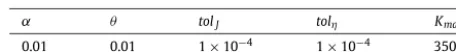
Table 1

Parametervaluesusedforthenumericalsimulations.

α θ tolJ tolη Kmax

0.01 0.01 1×10−4 _1×10−4 ₃₅₀₀

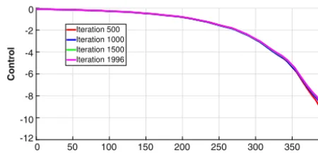
nondimensionalisedtimebetweensnapshotsandcouldinprincipleberelatedtoanacquisitiontimebetweenimagesgiven realbiological data.Foreachof theexperiments,apartfromthose ofSection 4.4, weset theinitial guessforthecontrol tobeconstantinspaceandtime(zero inthesingle cellcaseandoneforthemulti-cellexamples).Fortheapproximation ofthe forwardandadjoint equationswe used triangulations with8321 DOFs inall thesimulations, apart fromthoseof Section4.3,andselectedauniformtimestep

τ

=

1

×

10−3_{.Thesamenumericalparametersfortheoptimisationalgorithm} wereusedforalltheexperimentsandaregiveninTable 1.Ineveryexamplewereportonthealgorithmterminateddueto theupdateofthecontrolbeinglessthantheprescribedtolerance.

Thetechnicaldetailsofthehardwareusedtocarryoutthesimulationsare giveninRemark 4.1.

4.1.Remark(Hardwaredetails).Allthenumericalexperimentshavebeenperformedonthehighperformancecluster(HPC)at theUniversityofSussex.Eachofthesimulationswascarriedoutinserialusingasinglecoreofthecluster.TheHPCcluster currentlyconsistsof3140coreswithanevenmixtureofIntelandAMDCPUs.Themajorityoftheclusterare64coreAMD nodeswith256 GB RAM pernode, anda smallernumberof 512 GBRAM nodes.The clusteruses thehigh-performance Lustreclustered-filesystemforI/O,andcurrentlystandsat298TBofstorageforresearchuse.

4.2. Applicationtosyntheticdata

HereweapplythealgorithmtoasinglesyntheticcelldatasettakenfromthePhagoSightwebsitehttp://www.phagosight. org/synData.php.The syntheticcell was generatedasa mixtureofGaussianswithPoisson noisethat varied overtime to simulatethe displacementandchangeof shapeofa neutrophil asobservedin aZebrafish embryo.The dataforanalysis consisted of points on the synthetic cell membrane at a series of times (for simplicity we used 2d data, i.e., the cell membrane was a 1d curve embedded in

R

2_{). The initial and target curves we took as test data for the algorithm are} showninFig. 1(a).Toapply our algorithm,based ondiffuseinterface representations,we define the domain

:=

[

0

,

8

]

×

[

0

,

6

]

which was suchthat boththe initialandtarget curveswere containedinthedomain.We thenconstructed diffuse interface representationsofthe target datafollowingthe proceduredescribed in[5].Figs. 1(b) and1(c) showthe diffuse interface representations of the initial and target data respectively. In order to investigate the influence of the volume constraintonthecomputedcellmorphologiesweperformedtwoexperiments,inthefirstwesimplyconsideredtheforced Allen–Cahn modelfortheevolution withnovolume constraint, i.e.,(2.8) with

λ

=

0,andinthesecond we includedthe volume constraintas described in Section 2. The algorithm took 1996 iterations to meet the stopping criteria withno volume constraintand 2479iterations with thevolume constraint, corresponding to CPUtimesof 25 238and 119 216 s respectively.

Fig. 2showsthevalueoftheobjectivefunctionalagainstthenumberofiterationsoftheoptimisationalgorithmwithand withoutthevolumeconstraint. Weobservesimilarbehaviour inbothcaseswithaninitial rapiddecrease inthe objective functionalfollowedby amoregradualreduction witheach iterationasweapproachthe minimum.Fig. 3 showsthe zero level-set of thecomputed solution using the optimalcontrol atthe final time withand without the volume constraint. The curve corresponding to thezero level set isshaded by the value of thecomputed optimalcontrol. The background shading corresponds to the target data.In both casesthe position ofthe zero level-setof thecomputed solutionshows good agreement with the target data.Qualitatively we observe cells witha clearly defined “front” and “rear”, with the computedcontrolcorrespondingtoprotrusiveforcesatthefrontandcontractiveforcesattherear.

[image:8.561.155.368.53.224.2] [image:8.561.91.460.271.427.2]

Fig. 1.InitialandtargetdatafortheexampleofSection4.2.(Forinterpretationofthereferencestocolourinthisfigurelegend,thereaderisreferredto thewebversionofthisarticle.)

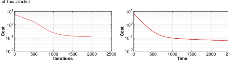
Fig. 2.ThevalueofthecostfunctionalversusthenumberofiterationsfortheexperimentsofSection4.2withandwithoutthevolumeconstraint.We observearapiddecreaseinthecostinitiallyfollowedbyamuchmoregradualdecreaseasweapproachtheminimum,thisisasexpectedsincethesteepest descentalgorithmisusedfortheupdateofthecontrol.

Fig. 8 showsthefidelityterm

ϕ

obs

(

x

)

−

ϕ(

x

,

T

)

k

_L2() withandwithoutthe volumeconstraintversus thenumberof iterations(wherekcorrespondstotheoptimisationiterationnumber).Thefidelitytermmaybeconsideredasaquantitative measureforthe“goodnessoffit”ofthecomputeddatatotheobservations.Weobserveasteadydecayinthefidelityterm asweapproachtheoptimalcontrolinbothcases.

4.3. Theeffectofmeshrefinement

[image:8.561.92.460.459.556.2]

[image:9.561.84.453.55.219.2] [image:9.561.137.404.284.415.2]

Fig. 3.Zerolevel-setofthesolutions(ϕ(x,T))computedusingtheapproximatedoptimalcontrol(η∗)withandwithoutthevolumeconstraintforthe experimentsofSection4.2.Thecurve(zerolevel-setofϕ(x,T))isshadedbytheapproximatedoptimalcontrol(η∗(x,T))andthebackgroundbythetarget data(ϕobs(x)).Thecolour-barcorrespondstothescaleforη∗(x,T).Weseegoodagreementbetweenthezerolevel-setofthedatacomputedwiththe optimalcontrolandthetargetdatainbothcases.(Forinterpretationofthereferencestocolourinthisfigurelegend,thereaderisreferredtotheweb versionofthisarticle.)

Fig. 4.AreaenclosedbythecellfortheexperimentsofSection4.2withandwithoutthevolumeconstraint.Thecellshrinksconsiderablyduringthe evolutionwithoutthevolumeconstraintwhilstagoodfittothelinearinterpolantoftheareaenclosedbythedataisobservedwiththevolumeconstraint.

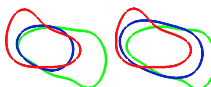
Fig. 5.Zerolevel-setsofthesolutionscomputed(ϕ(x,t))with theoptimalcontrol (η∗(x,t))fortheexperimentsofSection4.2withandwithoutthe volumeconstraintatt=0 (red),t=0.35 (blue)andt=0.4 (green).Weobservethatthevolumeenclosedbythebluecurveissignificantlysmallerthan thevolumesenclosedbytheredandgreencurveswithoutthevolumeconstraintwhilstthisisnotobservedifthevolumeconstraintisincluded.(For interpretationofthereferencestocolourinthisfigurelegend,thereaderisreferredtothewebversionofthisarticle.)

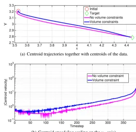
[image:9.561.83.454.454.607.2]

[image:10.561.131.414.48.321.2]

Fig. 6.Trajectoriesandspeedsofthecentroidofthezerolevel-setsofthesolutionwiththeoptimalcontrolwithandwithoutthevolumeconstraintfor theexampleofSection4.2.

totheobserveddata.Althoughinprincipleitwouldbeinterestingtoinvestigatetheinfluenceofrefiningboththetimestep andmesh-sizeonthecomputedresults,ourtestsindicatethatthealgorithmbreaksdownfortimestepssignificantlylarger than0

.

01 andhence,refinementofthetimestepandmesh-sizetogetherbecomescomputationallyprohibitive.

4.4. Theinfluenceoftheinitialguessforthecontrol

Here we applythealgorithm withthevolumeconstraintonthe simpleexampleofatranslatedcircletoillustrate the effect that the choice ofthe initial guess forthe control

η

hason the solution of the problem. To apply our algorithm we definethedomain

tobe

[−

3

,

6

]

× [−

3

,

3

]

witha triangulationof8321 gridpoints.We selectedauniformtimestep

τ

=

1

×

10−3andsettheinterfacialthickness

ε

=

0

.

1.Wetooktheend-timeT

=

0

.

8.Theremainingnumericalparameters for the optimisation algorithm are as givenin Table 1. The initial data was takento be a smoothed (byrunning a few steps ofthe Allen–Cahn solver) versionof thefunction takingthevalue 1inside B1(0

,

0

)

(a circleofradius1 centredat theorigin)and

−

1 in

/

B1(0

,

0

)

.The targetdatawastakentobeasmoothed(byrunningafewsteps oftheAllen–Cahn solver) versionofthefunctiontakingthevalue1inside B1(3

,

0

)

and

−

1 in

/

B1(0

,

0

)

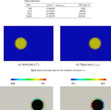
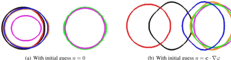
.Fig. 9showstheinitialandtarget diffuse interface data. To illustrate the effect of the choice of initial guesson the algorithm, we consider two different valuesfortheinitial guess,firstly weset

η

=

0 andsecondlywe set

η

=

c

· ∇

ϕ

,wherec

=

(

2

.

5

,

0

)

,i.e.,inthelattercase theinitialguessdependsonthesolutiontotheAllen–Cahnequation.Inbothcasesweusedthealgorithmwiththevolume constraints. Withthezeroinitial guessthealgorithm took 3262iterations tomeetthe stoppingcriteriacorresponding to a CPUtimeof320 433 s.Withthesecondchoice ofinitialguessthealgorithmtook 2056iterationsto meetthestopping criteriacorrespondingtoaCPUtimeof228 173 s respectively.

[image:11.561.158.383.84.192.2]

[image:12.561.91.460.55.162.2] [image:12.561.80.467.224.605.2]

Fig. 8.The value of the fidelity term versus the number of iterations for the experiments of Section4.2with and without the volume constraint.

Table 2 Meshrefinement.

DOFs ||ϕ(x,t)−ϕobs||L2() CPU time (s)

545 0.348165 3142

2113 0.176357 26 050

8321 0.154305 119 216

[image:12.561.160.386.228.277.2]

33 025 0.135178 291 597

Fig. 9.Initial and target data for the examples of Section4.4.

[image:12.561.76.472.474.652.2]

[image:13.561.74.470.55.158.2]

Fig. 11.Zerolevel-setsofthesolutionscomputed(ϕ(x,t))withtheoptimalcontrol(η∗(x,t))fortheexperimentsofSection4.4att=0 (red),t=0.2 (black),t=0.6 (blue),t=0.7 (orange),t=0.789 (pink)andt=0.8 (green).Weobservethenucleationofaphaseandachangeintopologywiththezero initialguesswhilsttherearenoevidentchangesintopologyandthezerolevel-setmaintainsafixedtopologyinthecaseofthenonzeroinitialguess.(For interpretationofthereferencestocolourinthisfigurelegend,thereaderisreferredtothewebversionofthisarticle.)

Fig. 12.AreaenclosedbythecurvefortheexperimentsofSection4.4.Agoodfittothelinearinterpolantoftheareasisonlyobservedwiththenonzero initialguess.Weobservearapidincreaseintheareaneartheendtimeforthezeroinitialguess,thiscorrespondstothetimeatwhichanewphaseis nucleated,cf.,Fig. 11(a).

4.5. Applicationtomulti-cellimagedatasets

Wenowapply thealgorithmto thecaseofmulti-cellimage datasets.Asa proof-of-conceptweconsiderthe simplest possiblescenariowherewehaveaninitialanddesireddataset bothconsistingoftwocellsthatarewellseparated.

Forthefirstexperimentwedefinedtheinitialdataandtarget dataasfollows.Definingthedomain

tobe

[−

2

,

8

]

×

[−

2

,

2

]

wedefinedthesubdomains

1

,

2

,

3

and

4

tobethesimplyconnectedboundeddomainswithboundarycurves

1,

2,

3

and

4

definedby (thecurves

1,

2

and

3

and

4

arethezerolevel-sets ofthediffuseinterfacesshownin Figs. 13(a)and13(b)respectively)

1

:=

x

∈

|

x2₁

+

x2₂

−

0

.

82

+

0

.

1 sin

(

4x1)

+

0

.

1 sin

(

3x2)

=

0

,

2

:=

x

∈

|

_x1 2

−

2

2

+

(x

2

−

0

.

6

)

2

−

0

.

72

+

0

.

1 sin

5x1

2

+

0

.

3 sin

(

2x2)

=

0

,

3

:=

x

∈

|

(x1

−

0

.

4

)

2

+

(x2

−

0

.

5

)

2

−

0

.

82

+

0

.

1 sin

(

6x1)

+

0

.

1 sin

(

7x2)

=

0

,

4

:=

x

∈

|

_x1

2

−

2

.

5

2

+

(x2

−

1

)

2

−

0

.

72

+

0

.

1 sin

7x1

2

+

0

.

1 sin

(

1

.

5x2)

=

0

.

Wethensettheinitialandtarget datatobe asmoothed(byrunningafewstepsoftheAllen–Cahnsolver)version ofthe function

ϕ

0

=

1 forx

∈

1

∪

2,

−

1 forx

∈

/ (1

∪

2) ,

and

ϕ

obs

=

[image:13.561.137.406.210.343.2]

1 forx

∈

3

∪

4,

−

1 forx

∈

/ (3

∪

4) .

Fig. 13showstheinitialandtargetdiffuseinterfacedata.

Aspreviously,wecomparetheresultsofthealgorithmwithandwithoutthevolumeconstraint.Forthisexperiment,the algorithmtook2035iterationstomeetthestoppingcriteriawithnovolumeconstraintand2199iterationswiththevolume constraint,correspondingtoCPUtimesof28 608and105 750s respectively.

[image:13.561.61.403.482.571.2]

[image:14.561.63.473.41.419.2] [image:14.561.75.471.57.157.2]

Fig. 13.Initial and target data for the examples of Section4.5.

Fig. 14.Cost functional versus the number of iterations for the examples of Section4.5.

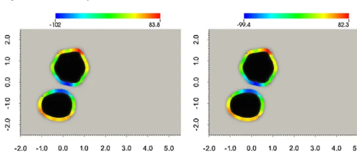
Fig. 15.Zerolevel-setofthesolutions(ϕ(x,T))computedusingtheapproximatedoptimalcontrol(η∗(x,t))withandwithoutthevolumeconstraintfor theexamplesofSection4.5.Thecurve(zerolevel-setofϕ(x,T))isshadedbytheapproximatedoptimalcontrol(η∗(x,T))andthebackgroundbythe targetdata(ϕobs(x)).Thecolour-barcorrespondstothescaleforη∗(x,T).Weseegoodagreementbetweenthezerolevel-setofthedatacomputedwith theoptimalcontrolandthetargetdatainbothcases.(Forinterpretationofthereferencestocolourinthisfigurelegend,thereaderisreferredtotheweb versionofthisarticle.)

the final time withandwithout the volumeconstraint shaded bythe value ofthe control withthe backgroundshading corresponding to thetarget data.Theresultsare similarto thesingle cellsimulations ofSection 4.2withan initialrapid decrease in the cost followed by a subsequent gradual decrease. The cells (zero level-sets) computed with the optimal control show good agreementwiththe targetdata forboth versionsofthealgorithm andforboth cells. Foreachof the versionsofthealgorithm,bothofthecomputedcellsagainpossesaclearlydefined“front”and“rear”similartothesingle cellcase.

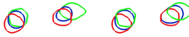
Fig. 16showstheareaenclosedbythezero-levelsetofthecomputedsolutionwiththeoptimalcontrolwithandwithout thevolumeconstrainttogetherwiththelinearinterpolantoftheareasofthedata.Weobserveanalogousbehaviourtothe singlecell.Intermsofthecomputedcellmorphologies,Fig. 17showssnapshotsofthecomputedzerolevel-setsforthetwo differentversionsofthealgorithm.Weseethatinthismulti-cellsettingthealgorithmhasimplicitlysolved thematching problembygeneratingtwodisjointcells whosetopologyremainsfixedthroughouttheevolution.Weobservethattheloss of volumein thecaseofnovolume constraintcorresponds toone ofthe cells intheintermediate snapshot (blue curve) enclosingamuchsmallerarea.

4.6. Anexamplewithtopologicalchange

[image:14.561.86.460.190.284.2] [image:14.561.72.474.315.434.2]

[image:15.561.136.407.56.184.2] [image:15.561.90.450.235.306.2]

Fig. 16.AreaenclosedbythecellfortheexperimentsofSection4.5withandwithoutthevolumeconstraint.Aswiththesinglecelldata,thearea(now thesumoftheareaofthetwocells)shrinksconsiderablyduringtheevolutionwithoutthevolumeconstraintwhilstagoodfittothelinearinterpolantof theareaenclosedbythedataisobservedwiththevolumeconstraint.

Fig. 17.Zerolevel-setsofthesolutionscomputedwiththeoptimalcontrolfortheexamplesofSection4.5withandwithoutthevolumeconstraintatt=0 (red),t=0.35 (blue)andt=0.4 (green).Thevolumeenclosedbybothcellsshrinksduringtheevolutionwithoutthevolumeconstraintwhilstthisisnot observedifthevolumeconstraintisincluded.Bothwithandwithoutthevolumeconstraint,theimplicitsolutionofthematchingprobleminthiscase generatestwodisjointcellswhichdonotchangeintopology.(Forinterpretationofthereferencestocolourinthisfigurelegend,thereaderisreferredto thewebversionofthisarticle.)

Definingthedomain

tobe

[−

2

,

6

.

3

]

× [−

2

.

5

,

2

.

5

]

wedefinedthesubdomains

1

,

2

,

3

and

4

tobethesimply connectedboundeddomainswithboundarycurves

1,

2,

3

and

4

definedby(seeFig. 18)

1

:=

x

∈

|

x2₁

+

x2₂

−

0

.

92

+

0

.

1 sin

(

4

.

5x1)

+

0

.

11 sin

(

3x2))

=

0

,

2

:=

x

∈

|

(x

1

−

5

)

2

+

x22

−

0

.

72

+

0

.

1 sin

5x1

2

+

0

.

3 sin

(

2x2

)

=

0

,

3

:=

x

∈

|

(x1

−

0

.

35

)

2

+

(x2

−

0

.

7

)

2

−

0

.

82

+

0

.

1 sin

(

6x1)

+

0

.

1 sin

(

7x2)

=

0

,

4

:=

x

∈

|

(x

1

−

0

.

3

)

2

+

(x

2

−

1

.

1

)

2

−

0

.

72

−

0

.

1 sin

7x1

2

+

0

.

1 sin

(

1

.

5x2

)

=

0

.

Wethensettheinitialandtarget datatobe asmoothed(byrunningafewstepsoftheAllen–Cahnsolver)version ofthe function

ϕ

0

=

1 forx

∈

1

∪

2,

−

1 forx

∈

/ (1

∪

2) ,

and

ϕ

obs

=

1 forx

∈

3

∪

4,

−

1 forx

∈

/ (3

∪

4) .

Fig. 18showstheinitialandtargetdiffuseinterfacedata.

Aspreviously,wecomparetheresultsofthealgorithmwithandwithoutthevolumeconstraint.Forthisexperiment,the algorithmtook1960iterationstomeetthestoppingcriteriawithnovolumeconstraintand1937iterationswiththevolume constraint,correspondingtoCPUtimesof27 553and93 150 s respectively.

Fig. 19showsthevalueoftheobjectivefunctionalagainstthenumberofiterations oftheoptimisationalgorithmwith andwithoutthevolumeconstraint.Fig. 20showsthezerolevel-setofthecomputedsolutionusingtheoptimalcontrolat the final time withandwithout thevolume constraintshaded by the value ofthe control withthebackground shading corresponding tothe targetdata.The resultsare similarto theprevious simulationswithan initial rapiddecreaseinthe costfollowedbyasubsequentgradualdecreaseandgoodagreementwiththetargetdataforbothversionsofthealgorithm andfor both cells. For each of theversions of the algorithm,both of the computedcells againposses a clearly defined “front”and“rear”.

[image:15.561.61.408.401.490.2]

[image:16.561.88.460.56.187.2] [image:16.561.92.458.214.310.2]

Fig. 18.Initial and target data for the examples of Section4.6.

Fig. 19.ThevalueofthecostfunctionalversusthenumberofiterationsfortheexamplesofSection4.6withandwithoutthevolumeconstraint.We observearapiddecreaseinthecostinitiallyfollowedbyamuchmoregradualdecreaseasweapproachtheminimum,thisisasexpectedsince the steepestdescentalgorithmisusedfortheupdateofthecontrol.

Fig. 20.Zerolevel-setofthesolutions(ϕ(x,T))computedusingtheapproximatedoptimalcontrol(η∗(x,t))withandwithoutthevolumeconstraintfor theexamplesofSection4.6.Thecurve(zerolevel-setofϕ(x,T))isshadedbytheapproximatedoptimalcontrol(η∗(x,T))andthebackgroundbythe targetdata(ϕobs(x)).Thecolour-barcorrespondstothescaleforη∗(x,T).Weseegoodagreementbetweenthezerolevel-setofthedatacomputedwith theoptimalcontrolandthetargetdatainbothcases.(Forinterpretationofthereferencestocolourinthisfigurelegend,thereaderisreferredtotheweb versionofthisarticle.)

constraint. Thismaybe due tothe change intopology of theinterface during theevolution. Fig. 22shows snapshotsof thecomputedzerolevel-setsforthetwodifferentversionsofthealgorithm.Unlikethepreviousexamplesweseethatfor thisparticularchoiceofinitialandtarget data,thealgorithmyieldscellswhichchangeintopologywithone ofthecurves shrinking untilitdisappearswhilsttheothersplits eventuallybecomingtwodisjointcurves.Thusouralgorithmgenerates trajectories correspondingto theannihilation (viashrinking)ofone cellwhilst theother cell splitsto formthetwo cells observedintheimagedataset.

4.7. Commentsonthenumericalexperiments

[image:16.561.90.457.357.513.2]

[image:17.561.136.407.55.184.2]

Fig. 21.AreaenclosedbythecellfortheexperimentsofSection4.6withandwithoutthevolumeconstraint.Aswiththesinglecelldata,thearea(now thesumoftheareaofthetwocells)shrinksconsiderablyduringtheevolutionwithoutthevolumeconstraint,whilsttheincorporationofthevolume constraintyieldsabetterfittothelinearinterpolantoftheareas.Unlikethepreviousexampleshowever,evenwiththevolumeconstraintthefittothe linearinterpolantoftheareasofthedataispoor.

Fig. 22.Zerolevel-setsofthesolutionscomputedwiththeoptimalcontrolfortheexamplesofSection4.6withandwithoutthevolumeconstraintatt=0 (red),t=0.3 (blue),t=0.396 (black)andt=0.4 (green).Weobservethatinthiscasethedifferencebetweenthetwoschemesislesspronounced.It isalsoclearthatbothwithandwithoutthevolumeconstraint,theimplicitsolutionofthematchingprobleminouralgorithminthiscaseleadstothe annihilationofonecell(asitshrinkstoapoint)whiletheothercellsplitswiththezerolevel-setchangingintopologyfromasingleclosedcurvetotwo disjointclosedcurves.(Forinterpretationofthereferencestocolourinthisfigurelegend,thereaderisreferredtothewebversionofthisarticle.)

approximatelyfourtimesaslong(intermsofCPUtime)asthosewithoutthevolumeconstraint.Thisisduetotheiterative nature ofthe algorithm usedto compute the Lagrange multiplier cf., Appendix A whichnecessitates multiple solves per timestep.WenotethattheCPUtimesofthealgorithmsmaybetoolargeformanyapplications.Inlightofthiswemention thatthestoppingcriteriawehaveusedmaybetoostrictformanyapplicationsandthatasignificantdecreaseinthecost functiontogetherwithareasonablefittothedataisobservedafterasfewas50iterations(whichreducestheCPUtimeby afactorofaround40)andthatformanyapplicationsthisleveloffitmaybesufficienthencethestoppingcriteriacouldbe relaxed.Finally wementionthatthecurrentsolutionprocedurebasedonuniformgrids andserialsolutionoftheforward andadjointproblemsmaybeimprovedandwearecurrentlyinvestigatingcombiningadaptivegridswithaparallelsolver fortheforwardandadjoint problemswhich givesa significantspeed upbutpresentsnewtechnicalchallengeswhichwe wishtoavoidinthispapertomaintainclarityofexposition.

5. Conclusion

Inthisstudywepresentedafirststeptowardsthedevelopmentofcelltrackingalgorithmsbasedonphysicalmodelsfor cellmigration.Thepresentedalgorithmseekstotrackwholecellmorphologiesandisapplicabletosinglecellormulti-cell image datasets.Ourapproachmaybe regardedasamodelfittingprocedureinwhichaphysicallyderived modelforthe evolutionofthecellorcellsisfittedtoexperimentalimagedatasets.Thealgorithmisbasedonthetheoryofoptimal con-trolofPDEsandfulldetailsofthederivationandimplementationofthealgorithmaregiven.Wealsopresentanumberof numericalexperimentsillustratingtheperformanceofthealgorithmwithsyntheticrepresentativesinglecellandmulti-cell imagedatasets.

[image:17.561.75.456.240.340.2]

tracking procedure. We illustrate thisfact by includingvolume conservation in themodel. Comparingthe results ofthe trackingalgorithmwithandwithoutvolumeconservation,weobserve,thatinanumberofsimulationsneglectingvolume conservationleadstophysicallyunrealisticcellmorphologieswithasignificantreductionofthecellvolumeintherecovered morphologies whilstthisundesirable effectisnolongerevident ifvolumeconservationisincluded.Wenote thatvolume conservation is more physically relevant in three dimensions. This is since large changes in volume in two-dimensional imaging data of cells (i.e., the area of the projections ofthe cell on to a two-dimensional plane) are often observed in experimentaldatadespitethecellsconservingtheirenclosed(three-dimensional)volume.

Of course volume conservationis only an exampleof the kindof biologyorphysics one maywish to encode in the algorithm. A numberof models that fitinto our framework havebeen proposed incorporating morecomplex biophysics such asspontaneous curvatures [9], forHelfrichtype models, adhesionforthe migration ofcells on substratesorin the ECM[13],cell–cellorcell–obstacleinteractions[4]andchemotaxis[12],thesemodelsarethuspotentialcandidatesforthe modeldrivingtheevolutioninourtrackingalgorithm.

Weworkwithdiffuseinterfacerepresentationsofthecellmembranetomakeuseofthematuretheoryfortheoptimal control ofsemilinearPDEs.Oneattractiveaspectofthisapproachisthat,aswedonotrequiresharpinterface representa-tionsofthecellmembrane,itmaybepossiblethereforetoworkdirectlywiththerawexperimentalimagedatasetwithout anyneed forsegmentation.However thediffuseinterface orphase field frameworkwe employ doesmakethealgorithm computationallyintensiveasevidencedbytherelativelylargeCPUtimesforourexperimentsandakeyareaforfuturework istoinvestigateimprovementsinthecomputationalefficiencyofthealgorithm.Thisneedisespeciallyevidentifonewishes to trackcells in3d,asalthoughourtheoretical frameworkappliesequallyto thissettingthecomputational costbecomes prohibitive.Computationalaspectsunderinvestigationinclude

•

Spatial andtemporal adaptivity which is challenging in thissetting asthe solution of the state equation enters the adjointequation.

•

Alternativeupdateschemesforthecontroltothesimpleyetrobustgradientbasedupdateconsideredinthisstudy.

•

Parallelisationandthedevelopmentoffastsolversforthesolutionofthestateandadjointequations.

Our initial numerical investigations suggest that with a combination of the techniques outlined above it is possible to efficiently track3dcell migrationandwe reporton thiselsewhere. Otherpotentially attractivedirectionsforfuturework wouldbe toconsiderhigherorderfiniteelement spacesforthediscretisation oftheforwardandadjointproblemsorthe use ofspectralelement methods,both ofwhichmayallow amoreaccurate solutionofthe forwardandadjointproblem withfewerdegreesoffreedom,hencereducingthememoryrequirements.

Investigatingtheperformanceofthealgorithmwithrealbiologicaldatafordifferentcelltypesandindifferent environ-ments isanimportantandworthwhiletask.Wearecurrentlyapplyingthealgorithmtothetrackingofinvivoneutrophil migration andintend to report on thiselsewhere. As mentioned previously one interpretation ofthe forcing

η

∗ isthat it accountsfor both protrusive forcesgenerated by polymerisation ofactin atthe leading edge ofthe cell together with contractileforcesgeneratedbytheactionofmyosinmotorsatthecellrear.Thusapotentialavenueforassessingthe plau-sibilityofthecelltrackscomputedwithouralgorithmwouldbetocomparethecomputed

η

∗ withexperimentalimaging dataon thelocationofpolymerisedactin andmyosin-II onthecellmembranewiththeexpectationbeingthatregions in which the computed forcing

η

∗ is positive wouldcorrespond to regions rich in polymerised actin andregions in which thecomputedforcing

η

∗ isnegativewouldcorrespondtoregionsrich inmyosin-II.Therearealsomanyextensionsofour approach whichare likelyto proveusefulin applications.Ouralgorithmcould equallybe applied tothe identificationof (possibly time-dependent)parametersinmodelsforcellmigration(e.g.,aspatiallyconstantforcingormaterialparameters suchassurfacetensionorbendingrigidity)howeverinthiscaseitislikelythatthesharpinterfaceapproachweproposein [5]willbemoreefficient.Asobservedinsomeoftheexperimentswereporton,theframeworkweemployallowschanges intopology ofthecells.Whilstthismaybedesirableforsomeapplications,e.g.,trackingcellsbeyondcelldivision orcell fusion,inmanybiologicalexperimentsthetopologyofthecells isfixed.Ourexperimentssuggestthat topologicalchanges ariseprimarilyinthecaseofmulti-cellimagedatasets.Inthissettingitshouldbepossibletotracktheevolutionofcertain topologicalinvariants(ormorespecificallydiffuseinterfacerepresentationsofsuchinvariants)andusetheseasanindicator forwhenthecomputedcellsarechangingintopology.Theusercouldthenmanuallyreducethemulti-celltrackingproblem tomultiplesinglecell(orsmallerscalemulti-cell)trackingproblemsbyspecifyingthecorrespondencebetweencellsin dif-ferentframes,withthehopethatchangesintopologydonotoccurforthesenewproblems.Themodelweproposeforthe evolutioninthisstudyisasimplificationofmoregeneralphysicallyrelevantmodelsinwhichbulkorsurfacePDEsforthe biochemistry arecoupledtoageometricevolutionlawforthemotion.Animportantareaforfutureworkistheextension oftheframeworktothismoregeneralsetting.Wenotethatthephasefieldapproachweemploymakesitcomputationally straightforward tocouplethegeometric evolutionlawforthemotiontobulkPDEs (posedeitherwithinthecellorinthe extra-cellularmatrix)[10,8,13].

Acknowledgements

This work (A.M., V.S. and C.V.) is supported by the Engineering and Physical Sciences Research Council, UK grant (EP/J016780/1)andtheLeverhulmeTrust ResearchProjectGrant(RPG-2014-149).K.B.was partiallysupportedbythe Em-birikionFoundation Grant(2011-2014)–Greece.Thecomputationswerecarriedoutusingthecomputationalresourcesof theSchoolofMathematicsandPhysicalSciences attheUniversityofSussex.Theonlydataassociatedwiththearticlewas obtainedfromthephagosightwebsite,www.phagosight.org,andisfreelyavailableforgeneraluse.

Appendix A. Numericalsolutionoftheforwardandadjointproblems

A.1. Discretisationofthestateequation

We introduce the variational formfor theforward problem(2.8) definedasfollows. Find

(ϕ,

λ)

∈

L2(

[

0

,

T

];

H1

())

×

L2

₍

₀

_,

_T

₎

_suchthat

∂

t

ϕψd

x

+

∇

ϕ

· ∇

ψd

x

=

1

ε

(c

G

η

−

λ)ψd

x

−

1

ε

2

G

(ϕ)ψd

x

∀

ψ

∈

H1

().

Let

T

be a decomposition of

intosimplexes (for simplicitywe assume

is polygonal). We define thefinite element space

V

:= {

ψ

h

∈

H1

()

∩

C0

()

:

ψ

h

|

k

∈

P

1

∀

k

∈

T

}

.

(A.1)

Forthe time discretisationwe employ an implicit–explicit methodwherethe diffusiveterm istreatedimplicitlyandthe reactiontermsexplicitly.Introducingtheshorthandforatimediscretesequence fn

:=

f

(

tn

)

andauniformtimestep

τ

with

T

=

M

τ

,

M

∈

N

,thefullydiscreteschemereads,forn

=

0

,

. . . ,

M

−

1,given

ϕ

n h

,

η

n

h

∈

V

find

(ϕ

n+1 h

,

λ

n+1

₎

_∈

_V

_×

_R

_suchthat

1

τ

(ϕ

n_h+1

−

ϕ

n_h

)ψ

hdx

+

∇

ϕ

_hn+1

· ∇

ψ

hdx

=

1

ε

(c

G

η

hn

−

λ

n+1

)ψ

hdx

−

1

ε

2

h

(G

(ϕ

_hn

))ψ

hdx

∀

ψ

h

∈

V

,

where

h

:

C0

()

→

V

denotestheLagrangeinterpolant.

Wesolvetheaboveproblemusingtheiterativetechniqueintroducedandstudiedin[21],whichusesabisectionmethod fortheLagrangemultiplier.Inparticularweseekaniterativesequence

{

φ

_hn+1,k

,

λ

n+1,k

}

k≥1where

φ

_hn+1,k solves

1

τ

(ϕ

n_h+1,k

−

ϕ

_hn

)ψ

hdx

+

∇

ϕ

_hn+1,k

· ∇

ψ

hdx

=

1

ε

(c

G

η

_hn

−

λ

n+1,k

)ψ

hdx

−

1

ε

2

h

(G

(ϕ

n_h

))ψ

hdx

∀

ψ

h

∈

V

,

with

λ

n+1,1

_{= −}

2ε τ

+

1,

λ

n+1,2

₌

2ε

τ

−

1 and

{

λ

n+1,k+1

_}

k≥2 satisfying

λ

n+1,k+1

=

λ

n+1,k

+

λ

n+1,k

−

λ

n+1,k−1 M_ϕn+1

−

[

ϕ

_hn+1,k

]

+

[

ϕ

n+1,k h

]

+

−

[

ϕ

n+1,k−1

h

]

+

,

wherewerecall

Mn_ϕ+1

:=

[

ϕ

0_h

]

₊

+

(n

+

1

)τ

T

[

ϕ

obs

]

+

− [

ϕ

h0

]

+

dx.

Wedeemthisiterationtohaveconvergedwhen

|

λ

n+1,k+1

−

λ

n+1,k

|

<

tol.

Thediscretisationoftheforwardproblemwithoutthevolumeconstraintisasabovewith

λ

=

0.Forthediscretisationof theadjointproblemweemployastandardsemi-implicitfiniteelementapproximation.

References

[1]D.Bray,CellMovements:FromMoleculestoMotility,Routledge,2001.

[2]Y.Xiong,P.A.Iglesias,Toolsforanalyzingcellshapechangesduringchemotaxis,Integ.Biol.2 (11–12)(2010)561–567. [3]E.Meijering,O.Dzyubachyk,I.Smal,Methodsforcellandparticletracking,MethodsEnzymol.504(2012)183.

[4] C.M.Elliott,B.Stinner,C.Venkataraman,Modellingcellmotilityandchemotaxiswithevolvingsurfacefiniteelements,J.R.Soc.Interface9 (76)(2012) 3027–3044,http://rsif.royalsocietypublishing.org/content/9/76/3027.abstract.

[5] W.Croft,C.M.Elliott,G.Ladds,B.Stinner,C.Venkataraman,C.Weston,Parameteridentificationproblemsinthemodellingofcellmotility,J.Math. Biol.(2014)1–38,http://dx.doi.org/10.1007/s00285-014-0823-6.

[6]F.Haußer,S.Rasche,A.Voigt,Theinfluenceofelectricfieldsonnanostructures—simulationandcontrol,Math.Comput.Simul.80 (7)(2010)1449–1457. [7]F.Haußer,S.Janssen,A.Voigt,Controlofnanostructuresthroughelectricfieldsandrelatedfreeboundaryproblems,in:ConstrainedOptimizationand

[8]D.Shao,W.Rappel,H.Levine,Computationalmodelforcellmorphodynamics,Phys.Rev.Lett.105 (10)(2010)108104.

[9]W.Marth,A.Voigt,Signalingnetworksandcellmotility:acomputationalapproachusingaphasefielddescription,J.Math.Biol.(2013)1–22. [10]F.Ziebert,S.Swaminathan,I.Aranson,Modelforself-polarizationandmotilityofkeratocytefragments,J.R.Soc.Interface9 (70)(2012)1084–1092. [11]M.Neilson,J.Mackenzie,S.Webb,R.Insall,Modellingcellmovementandchemotaxispseudopodbasedfeedback,SIAMJ.Sci.Comput.33 (3)(2011)

1035–1057.

[12]M.Neilson,D.Veltman,P.vanHaastert,S.Webb,J.Mackenzie,R.Insall,Chemotaxis:afeedback-basedcomputationalmodelrobustlypredictsmultiple aspectsofrealcellbehaviour,PLoSBiol.9 (5)(2011)e1000618.

[13]D.Shao,H.Levine,W.-J.Rappel,Couplingactinflow,adhesion,andmorphologyinacomputationalcellmotilitymodel,Proc.Nat.Acad.Sci.109 (18) (2012)6851–6856.

[14]K.M.Henry,L.Pase,C.F.Ramos-Lopez,G.J.Lieschke,S.A.Renshaw,C.C.Reyes-Aldasoro,Phagosight:anopen-sourceMATLAB®packagefortheanalysis offluorescentneutrophilandmacrophagemigrationinazebrafishmodel,PLoSONE8 (8)(2013)e72636.

[15]L.Bosgraaf,P.vanHaastert,T.Bretschneider,Analysisofcellmovementbysimultaneousquantificationoflocalmembranedisplacementandfluorescent intensitiesusingquimp2,CellMotil.Cytoskelet.66 (3)(2009)156–165.

[16]R.A.Tyson,D.Epstein,K.Anderson,T.Bretschneider,Highresolutiontrackingofcellmembranedynamicsinmovingcells:anelectrifyingapproach, Math.Model.Nat.Phenom.5 (01)(2010)34–55.

[17]M.P.Neilson,J.A.Mackenzie,S.D.Webb,R.H.Insall,Useoftheparameterisedfiniteelementmethodtorobustlyandefficientlyevolvetheedgeofa movingcell,Integ.Biol.2 (11–12)(2010)687–695.

[18]M.Vierling,Parabolicoptimalcontrolproblemsonevolvingsurfacessubjecttopoint-wiseboxconstraintsonthecontrol–theoryandnumerical realization,InterfacesFreeBound.16 (2)(2014)137–173.

[19]F.Tröltzsch,Optimal ControlofPartialDifferentialEquations:Theory, MethodsandApplications,GraduateStudiesinMathematics,vol. 112,AMS Bookstore,2010.

[20]X.Chen,Generationandpropagationofinterfacesinreaction–diffusionsystems,Trans.Am.Math.Soc.334 (2)(1992)877–913.

[21]J.Blowey,C.Elliott,Curvaturedependentphaseboundarymotionandparabolicdoubleobstacleproblems,in:DegenerateDiffusions,Springer,1993, pp. 19–60.

[22]G.Bellettini,M.Paolini,AnisotropicmotionbymeancurvatureinthecontextofFinsler geometry,HokkaidoMath.J.25 (3)(1996)537–566. [23]M.Brassel,E.Bretin,Amodifiedphasefieldapproximationformeancurvatureflowwithconservationofthevolume,Math.MethodsAppl.Sci.34 (10)

(2011)1157–1180.

[24]Q.Du,C.Liu,X.Wang,Simulatingthedeformationofvesiclemembranesunderelasticbendingenergyinthreedimensions,J.Comput.Phys.212 (2) (2006)757–777.

[25]M.Hinze,R.Pinnau,M.Ulbrich,S.Ulbrich,OptimizationwithPDE Constraints,MathematicalModelling:TheoryandApplications,vol. 23,2009. [26]J.Snyman, PracticalMathematicalOptimization:AnIntroductiontoBasicOptimizationTheoryand ClassicalandNewGradient-BasedAlgorithms,

AppliedOptimization,vol. 97,Springer,2005.

[27]T.F.Chan,L.A.Vese,Activecontourswithoutedges,IEEETrans.ImageProcess.10 (2)(2001)266–277.

[28]D.Dormann,T.Libotte,C.J.Weijer,T.Bretschneider,Simultaneousquantificationofcellmotilityandprotein-membrane-associationusingactive con-tours,CellMotil.Cytoskelet.52 (4)(2002)221–230.