Planets and stellar activity : hide and seek in the CoRoT 7 system

(1)

Planets and stellar activity: hide and seek in the CoRoT-7 system

R. D. Haywood,

1

†

A. Collier Cameron,

1

D. Queloz,

2

S. C. C. Barros,

3

M. Deleuil,

3

R. Fares,

1

M. Gillon,

4

A. F. Lanza,

5

C. Lovis,

2

C. Moutou,

3

F. Pepe,

2

D. Pollacco,

6

A. Santerne,

3,7

D. S´egransan

2

and Y. C. Unruh

8

1_{SUPA, School of Physics and Astronomy, University of St Andrews, St Andrews KY16 9SS, UK} 2_{Observatoire de Gen`eve, 51 Ch. des Maillettes, CH-1290 Sauverny, Switzerland}

3_{Aix Marseille Université, CNRS, LAM (Laboratoire d’Astrophysique de Marseille) UMR 7326, F-13388 Marseille, France} 4_{Institut d’Astrophysique et de Géophysique, Université de Liège, Allée du 6 août 17, Bat. B5C, B-4000 Liège, Belgium} 5_{INAF-Osservatorio Astrofisico di Catania, via S. Sofia, I-78 - 95123 Catania. Italy}

6_{Department of Physics, University of Warwick, Coventry CV4 7AL, UK}

7_{Centro de Astrof´ısica, Universidade do Porto, Rua das Estrelas, P-4150-762 Porto, Portugal} 8_{Astrophysics Group, Blackett Laboratory, Imperial College London, London SW7 2AZ, UK}

Accepted 2014 July 2. Received 2014 June 30; in original form 2013 May 30

A B S T R A C T

Since the discovery of the transiting super-Earth CoRoT-7b, several investigations have yielded different results for the number and masses of planets present in the system, mainly owing to the star’s high level of activity. We re-observed CoRoT-7 in 2012 January with both HARPS and CoRoT, so that we now have the benefit of simultaneous radial-velocity and photometric data. This allows us to use the off-transit variations in the star’s light curve to estimate the radial-velocity variations induced by the suppression of convective blueshift and the flux blocked by starspots. To account for activity-related effects in the radial velocities which do not have a photometric signature, we also include an additional activity term in the radial-velocity model, which we treat as a Gaussian process with the same covariance properties (and hence the same frequency structure) as the light curve. Our model was incorporated into a Monte Carlo Markov Chain in order to make a precise determination of the orbits of CoRoT-7b and CoRoT-7c. We

measure the masses of planets b and c to be 4.73±0.95 and 13.56±1.08 M_⊕, respectively.

The density of CoRoT-7b is (6.61±1.72)(Rp/1.58 R⊕)−3g cm−3, which is compatible with

a rocky composition. We search for evidence of an additional planet d, identified by previous authors with a period close to 9 d. We are not able to confirm the existence of a planet with

this orbital period, which is close to the second harmonic of the stellar rotation at∼7.9 d.

Using Bayesian model selection, we find that a model with two planets plus activity-induced variations is most favoured.

Key words: techniques: radial velocities – stars: activity – stars: individual: CoRoT-7 – planetary systems.

1 I N T R O D U C T I O N

In 2009 July, L´eger et al. (2009) announced the discovery of the transiting planet CoRoT-7b with an orbital period of 0.85 d. At the time, it had the smallest exoplanetary radius ever measured, of 1.68±0.09 R_⊕.

Following this discovery, a four month intensive HARPS cam-paign was launched in order to measure the mass of CoRoT-7b.

_{Based on observations made with the HARPS instrument on the 3.6 m} telescope under the program ID 088.C-0323 at Cerro La Silla (Chile). †E-mail:[email protected]

The results of this run are reported in Queloz et al. (2009). They expected the radial-velocity (hereafter RV) variations to be heav-ily affected by stellar activity, given the large modulations in the CoRoT photometry. The star’s light curve (2008–2009 CoRoT run) shows modulations due to starspots of up to 2 per cent, which tells us that CoRoT-7 is more active than the Sun, whose great-est variations in irradiance recorded are of 0.34 per cent (Kopp &

Lean2011). Indeed, a few simultaneous photometric measurements

from the Euler Swiss telescope confirmed that CoRoT-7 was very spotted throughout the HARPS run. In order to remove the activity-induced RV variations from the data, Queloz et al. (2009) applied a pre-whitening procedure followed by a harmonic decomposition. For the pre-whitening, the period of the stellar rotation signal is

2014 The Authors

at University of St Andrews on December 8, 2014

http://mnras.oxfordjournals.org/

(2)

identified by means of a Fourier analysis, and a sine fitted with this period is subtracted from the data. This operation is applied to the residuals to remove the next strongest signal, and so on until the noise level is reached. All the signals detected with this method were determined to be associated with harmonics of the stellar rotation period, except two signals at 0.85 and 3.69 d. The RV signal at 0.85 d was found to be consistent with the CoRoT transit ephemeris, thus confirming the planetary nature of CoRoT-7b. Its mass was found to be 4.8± 0.8 M_⊕. In order to assess the nature of the signal at 3.69 d, Queloz et al. (2009) used a harmonic decomposition to create a high-pass filter: the RV data were fitted with a Fourier series comprising the first three harmonics of the stellar rotation period, within a time window sliding along the data. The length of this window (coherence time) was chosen to be 20 d, so that any signals varying over a longer time-scale are filtered out – starspots

typically have lifetimes of about a month (Hussain2002;

Schri-jver2002). The harmonically filtered data were found to contain a strong periodic signal at 3.69 d, which was attributed to the orbit of CoRoT-7c, another super-Earth with a mass of 8.4±0.9 M_⊕.

A few months later, Bruntt et al. (2010) re-measured the stellar radius with improved stellar analysis techniques, which led to a slightly smaller planetary radius for CoRoT-7b than initially found, of 1.58±0.10 R_⊕.

A separate investigation was later carried out by Lanza et al. (2010). The stellar induced RV variations were synthesized based on a fit to the CoRoT light curve, which was computed according

to a maximum entropy spot model (Lanza et al.2009,2011). The

existence of the two planets was then confirmed by demonstrating that the activity-induced RV variations did not contain any spurious signals at the orbital periods of the two planets, with an estimated false alarm probability of less than 10−4_.

In another analysis, Hatzes et al. (2010) applied a pre-whitening procedure to the full width at half-maximum (FWHM), bisector span and CaIIH&K line emission derived from the HARPS spectra and cross-correlation analyses. These quantities vary according to activity only, and are independent of planetary orbital motions. No significant signals were found in any of these indicators at the periods of 0.85 and 3.69 d. Furthermore, they investigated the nature of a signal found in the RV data at 9.02 d. It had been previously detected by Queloz et al. (2009) but had been attributed to a ‘two frequency beating mode’ resulting from an amplitude modulation of a signal at a period of 61 d. This is close to twice the stellar rotation period so it was deemed to be activity related. Hatzes et al. found no trace of a signal at 9.02 d in any of the activity indicators. They thus suggest this RV signal could be attributed to a third planetary

companion with a mass of 16.7± 0.42 M_⊕. They also confirm

the presence of CoRoT-7b and CoRoT-7c, but find different masses than calculated by Queloz et al. (2009). This is inevitable since the derived masses of planets are intimately connected with the methods used to mitigate the effects of stellar activity on the RV data.

Hatzes et al. (2010,2011) developed a very simple method to remove stellar activity-induced RV variations, to obtain a more ac-curate mass for CoRoT-7b. The method relies on making several well-separated observations on each night, which was the case for about half of the HARPS data. Under the assumption that the varia-tions due to activity and other planets are negligible during the span of the observations on each night, it is possible to fit a Keplerian or-bit assuming that the velocity zero-point differs from night to night but remains constant within each night. Hatzes et al. (2010) report

a mass of CoRoT-7b of 6.9± 1.4 M_⊕ and the second analysis

(Hatzes et al.2011) yields a mass of 7.42±1.21 M_⊕, which is consistent.

Pont, Aigrain & Zucker (2010) carried out an analysis based

on a maximum entropy spot model (similar to Lanza et al.2010),

which makes use of many small spots as opposed to few large spots. The model is constrained using FWHM and bisector information. A careful examination of the residuals of the activity and planet models led to the authors to add an additional noise term in order to account for possible systematics beyond the formal RV uncertainties. Pont et al. (2010) argue that CoRoT-7b is detected in the RV data with much less confidence than in previous analyses, and report a mass of 2.3±1.8 M_⊕detected at a 1.2σlevel. Furthermore, they argued that the RV data are not numerous enough and lack the quality required to look for convincing evidence of additional companions. Boisse et al. (2011) applied theirSOAPtool (Boisse, Bonfils & Santos2012) to the CoRoT-7 system. This program simulates spots on the surface of a rotating star and then uses this model to compute the activity-induced RV variations of the star. With this technique, they obtain mass estimates for CoRoT-7b and CoRoT-7c. They judge that their errors are underestimated and suggest adding a noise term of 1.5 ms−1_{to account for activity-driven RV variations.} Their mass estimate for CoRoT-7b is in agreement with the value reported by Queloz et al. (2009) but they find a slightly higher value for the mass of CoRoT-7c.

Ferraz-Mello et al. (2011) constructed their own version of the high-pass filter employed by Queloz et al. (2009) in order to test the validity of this method and estimate masses for CoRoT-7b and 7c. They compared it to the method used by Hatzes et al. (2010,2011) and to a pure Fourier analysis. They concluded that the method is

robust, and obtained revised masses of 8.0±1.2 M_⊕for

CoRoT-7b and 13.6± 1.4 M_⊕ for CoRoT-7c, but make no mention of

CoRoT-7d.

The analysis by Lanza et al. (2010), which makes use of the

CoRoT light curve (L´eger et al.2009) to model the activity-induced RV variations, and those by Pont et al. (2010) and Boisse et al. (2011), which rely on the tight correlation between the FWHM and the simultaneous Euler photometry (Queloz et al.2009), could be much improved with simultaneous photometric and RV data (see Lanza et al., in preparation). The spot activity on CoRoT-7 changes very rapidly and it is therefore not possible to deduce the form of the activity-driven RV variations from photometry taken up to a year before the RV data. In the next section, we introduce the new simultaneous photometric and RV observations obtained in 2012 January with the CoRoT satellite and HARPS spectrograph. In Section 3, we describe our RV model which takes activity-induced RV variations into account by combining the method of Aigrain, Pont & Zucker (2012) and an additional RV Gaussian process (GP). Our model is implemented in Section 4, and we discuss the out-comes in Section 5.

2 O B S E RVAT I O N S

2.1 Photometry

CoRoT-7 (averageV-mag=11.67) was observed with the CoRoT

satellite (Auvergne et al.2009) from 2012 January 10 to March 29. Fig.1shows the part of the light curve which overlaps with the 2012 HARPS run. Measurements were taken in CoRoT’s high cadence mode (every 32 s). The data were reduced with the CoRoT imagette pipeline with an optimized photometric mask in order to maximize the signal to noise of the light curve. Further details on the data reduction are given by Barros et al. (in preparation). We binned the data in blocks of 0.07 d, which corresponds to 6176 s and is close to the orbital period of the satellite of 6184 s (Auvergne et al.2009)

(3)

[image:3.595.56.542.53.300.2] [image:3.595.309.548.344.464.2]

Figure 1. Upper panel: CoRoT-7 light curve over the span of the 2012 RV run, with our photometric fit at each RV observation overplotted as the blue curve. Lower panel: residuals of the fit.

Table 1. Transit information based on both CoRoT runs (preliminary results from Barros et al., submitted). Period 0.853 591 65±5.6×10−7d Transit ephemeris 2454398.07694±6.7×10−4HJD

in order to average the effects of all sources of systematic errors related to the orbital motion of CoRoT. A combined analysis of both CoRoT data sets is presented by Barros et al. (submitted). They derive the revised orbital period and epoch of first transit shown in Table1. These values will be used as prior information in our MCMC simulations (see Section 2).

2.2 Spectroscopy

The CoRoT-7 system was observed with the HARPS instrument

(Mayor et al.2003) on the ESO 3.6 m telescope at La Silla for

26 consecutive clear nights from 2012 January 12 to February 6, with multiple well-separated measurements on each night. The 2012 RV data were reprocessed in the same way as the 2008–2009 data (Queloz et al.2009) using the HARPS data analysis pipeline. The cross-correlation was performed using a K5 spectral mask. The

data are given in TableA1. The median, minimum and maximum

signal-to-noise ratio of the HARPS spectra at central wavelength 556.50 nm are 44.8, 33.8 and 56.2, respectively. Fig.2shows the RV variations of CoRoT-7 during the two campaigns. The RV variations during the second run have a smaller amplitude, implying that the star has become less active than it was in 2008–2009.

3 A M O D E L AC C O U N T I N G F O R S T E L L A R AC T I V I T Y

We model the RVs as the sum of two separate contributions: one from stellar activity, and one from one or more planets. The activity component makes use of the information contained within the light curve, and is described in Sections 3.1–3.4, while the planet(s) are

Figure 2. RV variations of CoRoT-7 measured with HARPS, during the (a)∼4 months 2008–2009 run, (b)∼1 month 2012 run. Note the difference in horizontal scale between the two panels.

assumed to follow Keplerian orbits. The overall model, described in Section 3.5, contains three free parameters controlling the amplitude of the different activity terms as well as five free parameters per planet. The manner in which we explore this parameter space and compare models with different numbers of planets is described in Section 4.

3.1 The FFmethod

Aigrain et al. (2012) found that RV variations induced by starspots are well reproduced by a model consisting of the product of the photometric fluxFand its first time derivativeF. It is assumed that the spots are small and limb-darkening is ignored. Spots influence the stellar RV by suppressing the photospheric surface brightness at the local rotational Doppler shift of the spot. Also, in areas of high magnetic field such as faculae, which on the Sun are associated with spot groups, the convective flow is inhibited, leading to an attenuation of the convective blueshift. This effect is thought to be the dominant contribution to the total RV signal in the Sun (Meunier, Desort & Lagrange2010).

(4)

As derived in Aigrain et al. (2012), the RV perturbationRVrot(t) to the star’s RV incurred by the presence of spots on the rotating photosphere can be expressed as follows:

RVrot(t)= − ˙

(t)

0

1−(t)

0

_R

∗

f , (1)

where(t) is the observed stellar flux,0is the stellar flux for a non-spotted photosphere and ˙(t) is the first time derivative of

(t).R_∗is the stellar radius. The parameterfrepresents the drop in flux produced by a spot at the centre of the stellar disc, and can be approximated as

f ≈ 0−min

0

, (2)

wheremin is the minimum observed flux, i.e. the stellar flux at maximum spot visibility.

The effect of the suppression of convective blueshift on the star’s RV produced by starspots and magnetized areas surrounding them is given by

RVconv(t)=

1−(t)

0

2_δV

cκ

f , (3)

whereδVcis the difference between the convective blueshift in the unspotted photosphere and that within the magnetized area, andκ is the ratio of this area to the spot surface (Aigrain et al.2012).

3.2 Evaluating theFFactivity basis functions

The flux at the time of each RV point has to be interpolated from the CoRoT light curve. In order to do this, we used a GP (Rasmussen & Williams2006; Gibson et al.2011). A GP is a non-parametric way to modelndata points. Its kernel is annxncovariance matrixKin which each element contains information about how much each pair of data are correlated with each other. The matrix is determined by a model covariance functionk(t,t) whose form reflects the quasi-periodic nature of the CoRoT light curve, as evolving active regions come in and out of view:

k(t, t)=η2

1exp

−(t−t)2 2η2

2

− 2 sin

2₍π(t−t)

η3 )

η2 4

. (4)

The terms η1 (amplitude of the GP), η2 (time-scale for growth

and decay of active regions), η3 (recurrence time-scale) andη4 (smoothing parameter) are the hyperparameters of k(t, t). The recurrence time-scale was set as the rotation period of the star, which we determined by computing the discrete autocorrelation function of the light curve (Edelson & Krolik1988). We found Prot=23.81±0.03 d, which is consistent with the estimate of L´eger et al. (2009) of about 23 d. The remaining three hyperparameters were estimated through a Monte Carlo Markov Chain (MCMC), training the GP by maximizing the likelihoodLof the GP fit to the CoRoT photometry. For a data sety(Rasmussen & Williams2006)

logL= −n

2log(2π)− 1

2log(|K+σ 2

i I|)

− 1 2y

T₍_K₊_σ2

i I)−1y, (5)

where|K|is the determinant of the covariance matrix and acts to penalize complex models. The first term is a normalization constant and the third term represents theχ2_{of the fit. We include an} ad-ditional white noise component through the termσ2

i I, whereσiis the error on each data pointyi(see TableA1) andIis the identity matrix.

The best value for the hyperparameter η2, which corresponds

to the time-scale for growth and decay of active regions is

η2=20.6±2.5 d, implying that the active regions on the stellar surface evolve on time-scales similar to the stellar rotation period. The fit is shown in the top panel of Fig.1. The residuals of the fit shown in the bottom panel show no correlated noise and have an rms scatter of 0.02 per cent. Once the covariance matrix has been calculated by training the GP on the data set, we can use this to interpolate the value of the stellar flux and of its first time derivative at the time of each RV data point, in order to calculateRVrot(t) andRVconv(t).

3.3 An additional activity basis function

The FFmethod is likely to provide an incomplete representation of activity-induced RV variations. For example, it does not consider the broad-band photometric effect of faculae that are not physically associated with starspots; Aigrain et al. (2012) assume that their effect onRVrotis quite small as they tend to have low photomet-ric contrast. Indeed, according to Lockwood et al. (2007), faculae become less important (relative to spots) in stars more active than the Sun. Faculae do, however, have a significant impact on the sup-pression of convective blueshift (Meunier et al.2010); indeed, we find that this effect dominates the total RV contribution induced by stellar activity (see Section 5.7). There are other phenomena that the FF method does not account for, such as∼50 ms−1_inflows towards active regions recently found on the Sun (Gizon, Duvall & Larsen2001; Gizon, Birch & Spruit2010). Such photospheric ve-locity fields may affect the RV curve even if they have no detectable photometric signature. In addition, some longitudinal spot distribu-tions have almost no photometric signature. They can nonetheless be incorporated in the RV model via a separate, flexible activity term that is not directly derived from the light curve.

We account for potential low-frequency signals not modelled by the FF terms by introducing an extra activity basis function that takes the form of a GP. This new GP, described by equation (6) below, represents an additional activity-driven RV signal, which we implicitly assume will have the same quasi-periodic covariance properties as the light curve. This GP is therefore governed by the following covariance function, with a set of hyperparametersθ:

k(t, t)=θ12exp

−(t−t)2 2θ2

2

−2 sin

2π(t−t)

θ3 θ2 4 . (6)

The amplitude of the GP,θ1is a free parameter in our total RV

model, as will be discussed in Section 3.5. The other hyperparam-eters,θ2,θ3andθ4are equal toη2,η3andη4, respectively. This equality arises from the assumption that the frequency structure of the covariance function representing the stellar activity should be the same for both the light curve and the RV curve. Please note that for the remainder of the paper, all references to a GP refer to that described by equation (6) unless otherwise specified.

3.4 Activity model

The total RV perturbationRVactivityinduced by stellar activity is then

RVactivity=ARVrot+BRVconv+RVadditional, (7)

whereAandBare scaling factors, and the amplitude ofRVadditional is controlled by the hyperparameterθ1of equation (6). In the present analysis,R_∗(which is needed to calculateRVrot) is set to the value

(5)

determined by Barros et al. (submitted). The values ofδVcandκ (needed forRVconv) are not known in the case of CoRoT-7 so they will be absorbed into the scaling constantB.

3.5 Total RV model

Our final model consists of the three basis functions for the stellar activity as well as a Keplerian signal for each one ofnplplanets

RVtot(ti)=RV0+RVactivity(ti, A, B, 0, θ1)

+

npl

k=1

Kk cos(νk(ti, tperi_k, Pk)+ωk)+ekcos(ωk)

, (8)

where RV0is a constant offset. The period of the orbit of planetk is given byPk, and its semi-amplitude isKk.νk(ti, tperi_k) is the true anomaly of planetkat timeti, andtperik is the time of periastron. Because it is difficult to constrain the argument of periastron for planets in low-eccentricity orbits, we introduce two parametersCk andSk (Ford2006). They are related to the eccentricityekof the planet’s orbit and the argument of periastronωkas follows:

Ck=√ek.cos(ωk), (9)

Sk=√ek.sin(ωk). (10)

The use of the square root imposes a uniform prior onek, reducing the bias towards high eccentricities typically seen when definingCk andSkasekcos (ωk) andeksin (ωk).

The eccentricity is defined as

ek=Sk2+Ck2, (11)

and the argument of periastron is

ωk =tan−1(Sk/Ck). (12)

4 A N A LY S I S

4.1 Periodogram analysis

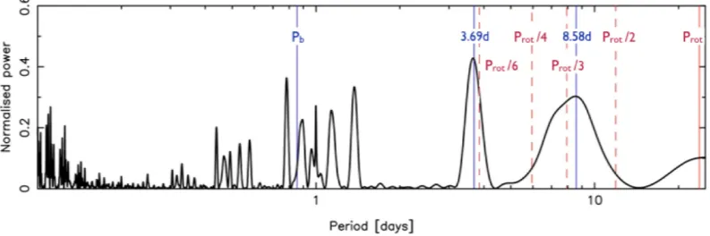
We produced a generalized Lomb–Scargle periodogram (Zechmeis-ter & K¨urs(Zechmeis-ter2009) of the 2012 RV data, shown in Fig.3. The stellar rotation period and its harmonics are marked by the red lines (solid and dashed, respectively). Because the orbital period of CoRoT-7b is close to 1 d, its peak in the periodogram is hidden amongst the aliases produced by the two strong peaks at 3.69 and 8.58 d. The

peak at 3.69 d matches the period for CoRoT-7c of Queloz et al. (2009). We see another strong peak at a period of 8.58 d, which is close to the period found by Lanza (in preparation) of 8.29 d for the candidate planet signal CoRoT-7d, and about half a day shorter than that determined by Hatzes (in preparation) based on the same data set. The periodogram shows that this peak is very broad and spans the whole 8–9 d range. Several stellar rotation harmonics are also present within this range, so at this stage it is not possible to conclude on the nature of this signal (this is discussed further in Section 5.3).

4.2 MCMC parameter fitting analysis

The strongest periodic signals identified in the periodogram analysis of Section 4.1 were used as a starting point for an MCMC simulation (although we found that the choice of starting points does not affect the outcome of the chains). This time, the orbit of CoRoT-7b was fitted as well.

4.2.1 Choice of priors

The priors adopted for each parameter are given in Table2. The

knee of the modified Jeffreys prior (Gregory2007) for the semi-amplitudes of the planets was chosen to be the mean estimated error of the RV observations (σRV). Such a prior acts as a uniform prior whenK σRV, and as a Jeffreys prior forKσRV. This ensures that the semi-amplitudes do not get overestimated in the case of a non-detection. We adopt the same modified Jeffreys prior for the amplitudesAandBof the FFbasis functions and the amplitude of the GP (θ1).θ1is naturally constrained to remain low through the calculation ofL. The orbital eccentricity of the innermost planet was constrained so that the planet’s orbit remains above the stellar surface, while we imposed a simple dynamical stability criterion on the outer planets by ensuring their eccentricities were such that the orbit of each planet does not cross that of its inner neighbour. We note that the epochs of inferior conjunction of the outer non-transiting planets (corresponding to mid-transit for a 90◦orbit) were constrained to occur close to the inverse variance-weighted mean date of the HARPS observations in order to ensure orthogonality with the orbital periods.

4.2.2 Procedure

[image:5.595.100.497.566.698.2]

At every step of the chain, parametersA,B,0,θ1, RV0, and the orbital elements of all planets are allowed to take a random jump

Figure 3. Generalized Lomb–Scargle periodogram of the 2012 RV data set. The stellar rotation fundamental,Prot, and harmonics are represented with solid

and dashed lines, respectively. Also shown are the orbital period of CoRoT-7b derived from the transit analysis of Barros et al. (submitted),Pb, and the periods

of the two strong peaks at 3.69 and 8.58 d.

(6)

[image:6.595.307.545.55.173.2]

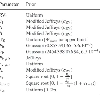
Table 2. Prior probability densities and ranges of the parameters modelled in the MCMC procedure. The knee of the modified Jeffreys prior is given in brackets. In the case of a Gaussian distribution, the terms within brackets represent the mean ¯xand stan-dard deviationσ. The terms within square brackets stand for the lower and upper limit of the specified distribution; if no interval is given, no limits were placed.

Parameter Prior

RV0 Uniform

θ1 Modified Jeffreys (σRV)

A Modified Jeffreys (σRV)

B Modified Jeffreys (σRV)

0 Uniform [max, no upper limit]

Pb Gaussian (0.853 591 65, 5.6.10−7)

t0b Gaussian (2454 398.076 94, 6.7.10−4)

Pk₌b Jeffreys

t0k=b Uniform

Kk Modified Jeffreys (σRV)

eb Square root [0,1−Rab∗]

ek₌b Square root [0,1−aka−k1(1+ek−1)] ωk Uniform [0,2π]

in parameter space. The unspotted flux level0is not allowed to take values less than the maximum observed flux. The two activity

functionsRVrotandRVconv are computed for every new value

of0. These two activity basis functions, together with the planet RVs and RV0are then subtracted from the data and the GP is fitted to the RV residuals. The hyperparametersθ2,θ3andθ4are kept fixed as they are better constrained by the light curve than the RVs, and computing them at each step of the MCMC would be

cumbersome. The likelihood Lof the RV residuals is calculated

at each step (according to equation 5) in order to decide whether this set leads to a better fit than the previous set. The step is then accepted or rejected, the decision being made via the Metropolis– Hastings algorithm (Metropolis et al.1953). It allows some steps to be accepted when they yield a slightly poorer fit, in order to

prevent the chain from becoming trapped in a localLmaximum

and instead explore the full parameter landscape. Once the burn-in

phase is complete, i.e.Lbecomes smaller than the median of all

previousL(Knutson et al.2008), the chain goes through 100 000 steps, over which the standard deviations of all the parameters are calculated. These define the jump lengths in each parameter for all subsequent transition proposals. The code goes through another 200 000 steps in order to explore the parameter landscape in the vicinity of the maximum ofL. This last phase provides the joint posterior probability distribution of all parameters of the model. The good convergence of the code was checked using the Gelman–

Rubin criterion (Gelman et al.2004; Ford2006), which must be

smaller than 1.1 to ensure that the chain has reached a stationary state.

5 R E S U LT S A N D D I S C U S S I O N

5.1 Justification for the use of a GP

We found that an RV model including a GP with a quasi-periodic covariance structure was the only model that would yield uncorre-lated, flat residuals. Regardless of the number of planets modelled, without the inclusion of this GP the residuals always display

cor-Figure 4. Top: RV residuals remaining after fitting a three-planet+FF activity functions model. They contain quasi-periodic variations, and show the need to use a red noise ‘absorber’ such as a GP. Bottom: RV residuals after including a GP with a quasi-periodic covariance function in our RV model. The rms of the residuals, now uncorrelated, is 1.96 ms−1_{which is at}

the level of the error bars of the data.

related behaviour. Fig.4shows the residuals remaining after fitting the orbits of CoRoT-7b, CoRoT-7c and a third Keplerian, and the two basis functions of the FF model. We see that even the addi-tion of a third Keplerian does not absorb these variaaddi-tions, which appear quasi-periodic. Also, we note that a GP with a less complex, square exponential covariance function does not fully account for correlated residuals in either a two- or three-planet model. A com-parison between a model with two planet orbits, the FFbasis func-tions and a GP that has square exponential or quasi-periodic covari-ance properties yields a Bayes factor of 3.106_{in favour of the latter.} This implies that the active regions on the stellar surface do remain, in part, from one rotation to the next.

5.2 Bayesian model selection

We ran MCMC simulations for models with 0 (activity only), 1 and 2 planets. The marginal likelihood of each model is estimated from the MCMC samples using the method of Chib & Jeliazkov (2001) (see Appendix A), and is listed in the second to last row of Table3. We also tested a three-planet model, which is discussed in Section 5.3.

The two-planet model is preferred over the activity-only and one-planet model (see the first three columns in Table3). It is also found that a two-planet model with free orbital eccentricities is preferred over a model with forced circular orbits by a Bayes’ factor of 5.103_. The model with forced circular orbits is penalized mostly because of the non-zero eccentricity of CoRoT-7c. Indeed, keepingebfixed to zero while lettingec free yields a Bayes’ factor of 270 (over a model with both orbits circular), while the Bayes’ factor between models with eb fixed or free (ec free in both cases) is only 36. A model with no planets, consisting solely of the FFbasis functions and a quasi-periodic GP (Model 0) is severely penalized; this attests that models with the covariance properties of the stellar activity do not absorb the signals of planets b and c.

5.3 9-d signal: CoRoT-7d or stellar activity?

We investigated the outputs of three-planet models in order to look for the 9-d signal present in the 2009 RV data (Queloz et al.2009; Hatzes et al.2010), whose origin has been strongly debated (cf. Section 1 and references therein).

First, we fitted a model comprising three Keplerians, the FFbasis functions and a GP with a quasi-periodic covariance function. We recover the two inner planets but do not detect another signal with

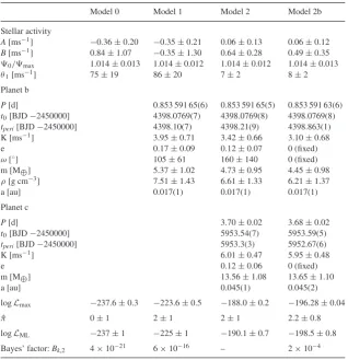
[image:6.595.82.246.154.311.2]

(7)

[image:7.595.139.458.121.451.2]

Table 3. Outcome of a selection of models: Model 0: stellar activity only, modelled by the FF basis functions and a GP with a quasi-periodic covariance function; Model 1: activity and 1 planet; Model 2: activity and 2 planets; Model 2b: activity and 2 planets with eccentricities fixed to 0.The numbers in brackets represent the uncertainty in the last digit of the value. Also given are the maximum likelihood (logLmax), the posterior ordinate ( ˆπ) and the marginal likelihood (logLML)

for each model. In the last row, each model is compared to Model 2 using Bayes’ factor.

Model 0 Model 1 Model 2 Model 2b

Stellar activity

A[ms−1] −0.36±0.20 −0.35±0.21 0.06±0.13 0.06±0.12 B[ms−1] 0.84±1.07 −0.35±1.30 0.64±0.28 0.49±0.35 0/max 1.014±0.013 1.014±0.012 1.014±0.012 1.014±0.013

θ1[ms−1] 75±19 86±20 7±2 8±2

Planet b

P[d] 0.853 591 65(6) 0.853 591 65(5) 0.853 591 63(6)

t0[BJD−2450000] 4398.0769(7) 4398.0769(8) 4398.0769(8)

tperi[BJD−2450000] 4398.10(7) 4398.21(9) 4398.863(1)

K [ms−1_] _3.95_±_0.71 _3.42_±_0.66 _3.10_±_0.68

e 0.17±0.09 0.12±0.07 0 (fixed)

ω[◦] 105±61 160±140 0 (fixed)

m [M_⊕] 5.37±1.02 4.73±0.95 4.45±0.98

ρ[g cm−3_] _7.51_±_1.43 _6.61_±_1.33 _6.21_±_1.37

a [au] 0.017(1) 0.017(1) 0.017(1)

Planet c

P[d] 3.70±0.02 3.68±0.02

t0[BJD−2450000] 5953.54(7) 5953.59(5)

tperi[BJD−2450000] 5953.3(3) 5952.67(6)

K [ms−1] 6.01±0.47 5.95±0.48

e 0.12±0.06 0 (fixed)

m [M_⊕] 13.56±1.08 13.65±1.10

a [au] 0.045(1) 0.045(2)

logLmax −237.6±0.3 −223.6±0.5 −188.0±0.2 −196.28±0.04

ˆ

π 0±1 2±1 2±1 2.2±0.8

logLML −237±1 −225±1 −190.1±0.7 −198.5±0.8

Bayes’ factor:Bk,2 4×10−21 6×10−16 – 2×10−4

any significance. The residuals are uncorrelated and at the level of the error bars. We then constrained the orbital period of the third planet with a Gaussian prior centred around the period recently reported by Tuomi et al. (2014) atPd=8.8999±0.0082 d, and

imposed a Gaussian prior centred at 2455949.97±0.44 BJD on

the predicted time of transit (which corresponds to the phase we determined based on the orbital period of Tuomi et al. 2014). We recover a signal which corresponds to a planet mass of 13±5 M_⊕ and is in agreement with the mass proposed by Tuomi et al. (2014).

However, the marginal likelihood of this model is−192.5±0.7;

this is lower than the marginal likelihood of the two-planet model

(Model 2, logLML= −190.1±0.7), which suggests that the

ad-dition of an extra Keplerian at 9 d is not justified in view of the improvement to the fit.

Since this orbital period is very close to the second harmonic of the stellar rotation, it is plausible that the GP could be absorbing some or all of the signal produced by a planet’s orbit at this period. In order to test whether this is the case, we took the residuals of Model 2 and injected a synthetic sinusoid with the orbital parameters of planet d reported by Tuomi et al. (2014). We fitted this fake data set with a model consisting of a GP (with the same quasi-periodic covariance function as before), a Keplerian and a constant offset. We find that the planet signal is completely absorbed by the Keplerian model, within uncertainties – the amplitude injected was

5.16±1.84 m.s−1_{, while that recovered is 4.97}_±_{0.35 m.s}−1_{. This} experiment attests that the likelihood of the model (see equation 5) acts to keep the amplitude of the GP as small as possible, in order to compensate for its high degree of flexibility, and allow other parts of the model to fit the data if they are less complex than the GP. We can thus conclude that if there were a completely coherent signal close to 9 d, it would be left out by the GP and be absorbed by the third Keplerian of the three-planet model.

This signal therefore cannot be fully coherent over the span of the observations. Indeed, we see in the periodogram of the RV data in Fig.3that the peak at this period is broad. We note that despite the lower activity levels of the star in the 2012 data set, the 9-d period is less well determined in this data set than in the 2008–2009 one. This peak is also broader than we would expect for a fully coherent signal at a period close to 9 d with the observational sampling of the 2012 data set. This is likely to be caused by variations in the phase and amplitude of the signal over the span of the 2012 data.

Based on the 2012 RV data set, we do not have enough evidence to confirm the presence of CoRoT-7d as its orbital period of 9 d is very close to the second harmonic of the stellar rotation. Furthermore, the period measured for the 2009 data set by Hatzes et al. (2010) Pd=9.021±0.019 d is not precise enough to allow us to determine whether the signals from the two seasons are in phase, as was

done in the case of αCentauri Bb by Dumusque et al. (2012).

(8)

The cycle count of orbits elapsed between the two data sets is: n = 1160/9.021 = 128.6 orbits. The uncertainty is n σPd/Pd=

n(0.019/9.021)=0.27 orbits. Although this 1σuncertainty is less than one orbit, it is big enough to make it impossible to test whether the signal is still coherent. The most likely explanation, given the existing data, is that the 8–9 d signal seen in the periodogram of Fig.3is a harmonic of the stellar rotation.

5.4 Best RV model: 2 planets+stellar activity

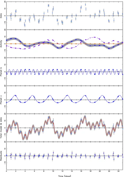
Fig.5shows each component of the total RV model plotted over the duration of the HARPS RV campaign. We see that the suppression of convective blueshift by active regions surrounding starspots has a much greater impact on RV than flux blocked by starspots; this is discussed further in Section 5.7.

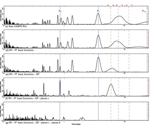
Fig.6shows Lomb–Scargle periodograms of the CoRoT 2012

light curve and the HARPS 2012 RV data. Panel (a) shows the periodogram of the full CoRoT 2012 light curve, while panel (b) represents the periodogram of the GP fit to the light curve sampled at the times of the HARPS 2012 RV observations. Both periodograms reveal a stronger peak atProt/2 than atProt, which indicates the presence of two major active regions on opposite hemispheres of the star. This is in agreement with the variations in the light curve in Fig.1. Given that suppression of convective blueshift appears to be the dominant signal, we would expect a similar frequency structure to be present in the periodogram of the RV curve (panel c). Indeed, we see that the stellar rotation harmonics bracket the 6–10 d peak in the periodogram, which has significantly greater power than the fundamental 23-d rotation signal. In panel (d), we remove the

two FF basis functions. We then subtract the GP (panel e). We

see that the GP absorbs most of the power present in the 6–10 d range. In panel (f), we have also subtracted the orbit of planet c.

This removes the peaks at Pc and its 1-d alias at ∼1.37 d. The

peak due to CoRoT-7b now stands out along with its 1-d alias at

P =1/(1−1/Pb)∼5.82 d and harmonicsPb/2 andPb/3. Finally, we subtract the orbit of planet b, and are left with the periodogram of the residuals. We see that no strong signals remain except at the 1- and 2-d aliases arising from the window function of the ground-based HARPS observations.

The posterior joint probability distributions of each pair of pa-rameters for the two-planet (free eccentricities) model are shown in Fig.7. There are no strong correlations between any of the parame-ters. TheKamplitudes of planets b and c are found to be unaffected by the number of planets, choice of eccentric or circular orbits, or choice of activity model (all, some or none of RVactivity), even when we leavePcunconstrained. The residuals, with an rms scat-ter of 1.96 ms−1_{are at the level of the error bars of the data (see} TableA1) and show no correlated behaviour, as seen in the bottom

panel of Fig. 4. The masses of planets b and c are presented in

Sections 5.5 and 5.6.

5.5 CoRoT-7b

The orbital parameters of CoRoT-7b are listed in the third column of Table3. The orbital eccentricity of 0.12±0.07 is detected with a low significance and is compatible with the transit parameters determined by Barros et al. (submitted). The phase-folded RV signal of CoRoT-7b is shown in Fig.8.

As mentioned in Section 5.2, the mass of CoRoT-7b is not affected by the choice of model, which attests to the robustness of this result.

Our mass of 4.73±0.95 M_⊕is compatible, within uncertainties,

with the results found by Queloz et al. (2009), Boisse et al. (2011)

and Tuomi et al. (2014). It is within 2σof the masses found by Pont et al. (2010), Hatzes et al. (2011) and Ferraz-Mello et al. (2011).

Using the radius found by Bruntt et al. (2010), CoRoT-7b is

found to be slightly denser than the Earth (ρ_{⊕ =}5.52 g cm−3_), withρb=6.61±1.72 g cm−3(see Table3). The reader should refer to Barros et al. (submitted) for a more detailed discussion of the density of CoRoT-7b.

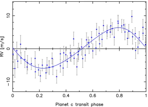
5.6 CoRoT-7c

We make a robust detection of CoRoT-7c at an orbital period of

3.70± 0.02 d, which is in agreement with previous works that

considered planet c. The phase-folded RV signal of CoRoT-7c is

shown in Fig. 9. We estimate its mass to be 13.56± 1.08 M_⊕

(see Table3). Our mass is in agreement with that given by Boisse et al. (2011) and Ferraz-Mello et al. (2011). It is just over 2σlower than the mass found by Hatzes et al. (2010), and over 3σ greater than the mass calculated by Queloz et al. (2009). It suggests that the harmonic filtering technique employed by Queloz et al. (2009) suppresses the amplitude of the signal at this period. This may be due to the fact thatPcis close to the fifth harmonic of the stellar rotation,Prot/6∼3.9 d (see Fig.3), but Queloz et al. (2009) only model RV variations using the first two harmonics, thus leaving PcandProt/6 entangled. Ferraz-Mello et al. (2011), who performed a similar analysis to that of Queloz et al. (2009), mention that the proximity ofPctoProt/6 may lead to underestimating the RV

amplitude of CoRoT-7c by up to 0.5 ms−1_{due to beating between}

these two frequencies.

We estimated the minimum orbital inclination this planet has to have in order to be transiting. Its radiusRc can be approximated using the formula given by Lissauer et al. (2011):

Rc=

_M

c

M_⊕

1/2.06

R_⊕, (13)

where M_⊕and R_⊕are the mass and radius of the Earth. Using the mass for CoRoT-7c given in the third column of Table3, we find

Rc=3.54 R⊕. With this radius, CoRoT-7c would have to have a

minimum orbital inclination of 83.7◦in order to be passing in front of the stellar disc with respect to the observer.

CoRoT-7b’s orbital axis is inclined at 79.0◦ to the line of

sight (preliminary result of Barros et al., submitted). According to Lissauer et al. (2011), over 85 per cent of observed compact plan-etary systems containing transiting super-Earths and Neptunes are coplanar within 3◦. We conclude that planet c is not very likely to transit. Indeed, no transits of this planet are detected in any of the CoRoT runs. We infer that any planets further out from the star with a similar radius or smaller are even less likely to transit.

5.7 The stellar activity of CoRoT-7

In Model 2, the rms scatter of the total activity model is 4.86 ms−1 (see Fig.5b). For moderately active host stars such as CoRoT-7, the activity contribution largely dominates the reflex motion induced by a closely orbiting super-Earth.

The rms scatter ofRVrotandRVconvare 0.46 and 1.82 ms−1, respectively. The smaller impact of the surface brightness inhomo-geneities on the RV variations could be due to the smallvsiniof the star (Bruntt et al.2010), because the amplitude of these vari-ations scales approximately withvsini(Desort et al.2007). This suggests that for slowly rotating stars such as CoRoT-7, the sup-pression of convective blueshift is the dominant contributor to the

(9)

[image:9.595.88.509.55.651.2]

Figure 5. Time series of the various parts of the total RV model for Model 2, after subtracting the star’s systemic velocity RV0. All RVs are in ms−1. Panel

(b):RVrot(orange full line),RVconv(purple dashed line) andRVadditional(blue full line with grey error band). Panel (e): the total model (red), which is

the sum of activity and planet RVs, is overlaid on top of the data (blue points). Subtracting the model from the data yields the residuals plotted in panel (f).

(10)

[image:10.595.50.544.242.656.2]

Figure 6. Lomb–Scargle periodograms of: (a) the full 2012 CoRoT light curve; (b) the GP fit to the 2012 CoRoT light curve sampled at the times of RV observations; (c) the raw 2012 HARPS RV observations; (d) the RV data, from which the FFbasis functions have been subtracted; (e) same as (d), with the GP also removed; (f) same as (e), with the signal of planet c removed; (g) same as (f), with planet b removed.

(11)

Figur e 7. Phase p lots for the MCMC chain of Model 2 for all parameters A , B , θ1 , 0 , RV 0 , Pb , t0b , Kb , √ e b sin ωb , √ e b cos ωb , Pc , t0c , Kc , √ e c sin ωc ,a n d √ e c cos ωc . P oints in y ello w , red and blue are w ithin the 1 , 2 and 3 σ confidence re g ions, respecti v ely . T he scale of each axis corresponds to the d eparture of each parameter from its v alue at m aximum lik elihood. All are expressed in p er cent except for Pb , t0b and t0c which are expressed as one part per m illion. The d istrib utions of 0 display a sharp cutof f at its minimum allo wed v alue, which corresponds to the m aximum observ ed fl ux v alue max .

(12)

[image:12.595.45.284.55.229.2]

Figure 8. Phase plot of the orbit of planet b for Model 2, with the contri-bution of the activity and planet c subtracted.

Figure 9. Phase plot of the orbit of planet c for Model 2, with the contri-bution of the activity and planet b subtracted.

activity-modulated RV signal, rather than the rotational Doppler shift of the flux blocked by starspots. This corroborates the findings of Meunier et al. (2010) and Lagrange, Desort & Meunier (2010), who showed that the suppression of convective blueshift is the dom-inant source of activity-induced RV variations on the Sun, which is also a slowly rotating star.

We use a GP to absorb correlated residuals due to other physical phenomena occurring on time-scales of order of the stellar rotation period. In the case of CoRoT-7, these combined signatures have an rms of 3.95 ms−1_{, suggesting that there are other processes than} those modelled by the FFmethod at play.

6 C O N C L U S I O N

The CoRoT-7 system was re-observed in 2012 with the CoRoT satellite and the HARPS spectrograph simultaneously. These

ob-servations allowed us to apply the FF method of Aigrain et al.

(2012) to model the RV variations produced by the magnetic activ-ity of CoRoT-7. This approach makes use of the star’s light curve and its first time derivative to model the rotational Doppler shift of the flux blocked by starspots, and the suppression of convective

blueshift occurring in active regions on the stellar surface. If we only use the FFmethod to model the activity, we find correlated noise in the RV residuals which cannot be accounted for by a set of Keplerian planetary signals. This indicates that some activity-related noise is still present. Indeed, the FF method does not ac-count for all phenomena such as the effect of limb-brightened facu-lar emission on the cross-correlation function profile, photospheric inflows towards active regions, or faculae that are not spatially as-sociated with starspot groups. Furthermore, some longitudinal spot distributions have almost no photometric signature. To model this low-frequency stellar signal, we use a GP with a quasi-periodic co-variance function that has the same frequency structure as the light curve.

We run an MCMC simulation and use Bayesian model selection to determine the number of planets in this system and estimate their masses. We find that the transiting super-Earth CoRoT-7b has a mass of 4.73±0.95 M_⊕. Using the planet radius estimated by Bruntt et al. (2010), CoRoT-7b has a density of (6.61±1.72)(Rp/1.58 R_⊕)−3 _{g cm}−3_{, which is compatible with a rocky composition.} We confirm the presence of CoRoT-7c, which has a mass of

13.56± 1.08 M_⊕. These findings agree with the analyses made

by Barros et al. (submitted), Hatzes et al. (in preparation), Lanza et al. (in preparation) and Tuomi et al. (2014).

We search for evidence of an additional planetary companion at a period of 9 d, as proposed by Hatzes et al. (2010) following an analysis of the 2008–2009 RV data set. While the Lomb–Scargle periodogram of the 2012 RVs displays a strong peak in the 6–10 d range, we find that this signal is more likely to be associated with the second harmonic of the stellar rotation at∼7.9 d.

In CoRoT-7, the RV modulation induced by stellar activity dom-inates the total RV signal despite the close-in orbit of (at least) one super-Earth and one sub-Neptune mass planet. Understanding the effects of stellar activity on RV observations is therefore crucial to improve our ability to detect low-mass planets and obtain a precise measure of their mass.

AC K N OW L E D G E M E N T S

We wish to thank the referee, S. Aigrain, for her recommendations that have greatly added to the rigour of this work. RDH acknowl-edges support from an STFC postgraduate research studentship. RF acknowledges support from STFC consolidated grant num-ber ST/J001651/1. SCCB acknowledges support by CNES, grant number 98761. AS acknowledges the support by the European Research Council/European Community under the FP7 through Starting Grant agreement number 239953. The CoRoT space mis-sion, launched on 2006 December 27, has been developed and is operated by CNES, with the contribution of Austria, Belgium, Brazil, ESA (RSSD and Science Programme), Germany and Spain. This research has made use of NASA’s Astrophysics Data System Bibliographic Services.

R E F E R E N C E S

Aigrain S., Pont F., Zucker S., 2012, MNRAS, 419, 3147 Auvergne M. et al., 2009, A&A, 506, 411

Boisse I., Bouchy F., H´ebrard G., Bonfils X., Santos N., Vauclair S., 2011, A&A, 528, A4

Boisse I., Bonfils X., Santos N. C., 2012, A&A, 545, 109 Bruntt H. et al., 2010, A&A, 519, A51

Chib S., Jeliazkov I., 2001, J. Am. Stat. Assoc., 96, 270

[image:12.595.45.285.279.452.2]

(13)

Desort M., Lagrange A. M., Galland F., Udry S., Mayor M., 2007, A&A, 473, 983

Dumusque X. et al., 2012, Nature, 491, 207 Edelson R. A., Krolik J. H., 1988, ApJ, 333, 646

Ferraz-Mello S., Tadeu dos Santos M., Beaug´e C., Michtchenko T. A., Rodr´ıguez A., 2011, A&A, 531, A161

Ford E. B., 2006, ApJ, 642, 505

Gelman A., Carlin J. B., Stern H. S., Rubin D. B., 2004, Bayesian Data Analysis. Chapman and Hall, London

Gibson N. P., Aigrain S., Roberts S., Evans T. M., Osborne M., Pont F., 2011, MNRAS, 419, 2683

Gizon L., Duvall Jr T., Larsen R., 2001, in Brekke P., Fleck B., Gurman J. B., eds, Proc. IAU Symp. 203, Recent Insights into the Physics of the Sun and Heliosphere. ASP, San Francisco, p. 189

Gizon L., Birch A., Spruit H., 2010, ARA&A, 48, 289 Gregory P. C., 2007, MNRAS, 381, 1607

Hatzes A. P. et al., 2010, A&A, 520, A93 Hatzes A. P. et al., 2011, ApJ, 743, 75 Hussain G., 2002, Astron. Nachr., 323, 349

Jeffreys S. H., 1961, The Theory of Probability. Oxford Univ. Press, Oxford Knutson H. A., Charbonneau D., Allen L. E., Burrows A., Megeath S. T.,

2008, ApJ, 673, 526

Kopp G., Lean J. L., 2011, Geophys. Res. Lett., 38, L01706 Lagrange A. M., Desort M., Meunier N., 2010, A&A, 512, A38 Lanza A. F. et al., 2009, A&A, 493, 193

Lanza A. F. et al., 2010, A&A, 520, A53

Lanza A. F., Boisse I., Bouchy F., Bonomo A. S., Moutou C., 2011, A&A, 533, A44

L´eger A. et al., 2009, A&A, 506, 287 Lissauer J. J. et al., 2011, ApJS, 197, 8

Lockwood G. W., Skiff B. A., Henry G. W., Henry S., Radick R. R., Baliunas S. L., Donahue R. A., Soon W., 2007, ApJS, 171, 260

Mayor M. et al., 2003, The Messenger, 114, 20

Metropolis N., Rosenbluth A. W., Rosenbluth M. N., Teller A. H., Teller E., 1953, J. Chem. Phys., 21, 1087

Meunier N., Desort M., Lagrange A. M., 2010, A&A, 512, A39 Pont F., Aigrain S., Zucker S., 2010, MNRAS, 411, 1953 Queloz D. et al., 2001, A&A, 379, 279

Queloz D. et al., 2009, A&A, 506, 303

Rasmussen C. E., Williams C. K. I., 2006, Gaussian Processes for Machine Learning. MIT Press, Cambridge, MA

Schrijver C. J., 2002, Astron. Nachr., 323, 157

Tuomi M., Anglada-Escud´e G., Jenkins J. S., Jones H. R. A., 2014, preprint (arXiv:1405.2016)

Zechmeister M., K¨urster M., 2009, A&A, 496, 577

A P P E N D I X A : M O D E L S E L E C T I O N

We ran MCMC chains for several different models and selected the best one using Bayesian statistics.

A1 Bayes’ factor

Given a data sety, consider two modelsMiandMj. In order to

determine which one is the simplest but still gives the best fit to the data, one can compare the two models by estimating their posterior odds ratio

P(Mi|y)

P(Mj|y) =

P r(Mi)

P r(Mj)·

m(y|Mi)

m(y|Mj),

(A1)

where the first factor on the right-hand side of the equation is the prior odds ratio. In this analysis, all models that are tested have the same prior information, so this ratio is just 1. This leaves us with the second part of the right-hand side of the equation. It is the ratio of the marginal likelihoodsmof each model, and is known as Bayes’ factor.

The marginal likelihoodmof a data setygiven a modelMiwith

a set of parametersθican be written as

m(y|Mi)=

f(y|Mi, θi)πi(θi|Mi) dθi, (A2)

wheref(y|Mi, θi) is the likelihood functionL. The termπi(θi|Mi)

accounts for the prior distribution of the parameters and can be incorporated as a penalty toL. According to Chib & Jeliazkov (2001), it is possible to write

m(y|Mi)= f(y|M_π i, θi)π(θi|Mi)

(θi|y,Mi) . (A3)

The denominatorπ(θi|y,Mi) is the posterior ordinate, which we

estimate using the posterior distributions of the parameters resulting from MCMC chains.

A2 Posterior ordinate

According to Chib & Jeliazkov (2001), the posterior ordinate ˆ

π(θi|y) can be evaluated by comparing the mean transition

proba-bility for a series ofMjumps from any givenθitoa referenceθ∗, to the mean acceptance value for a series ofJtransitionsfromθ_∗. This can be written as

ˆ

π(θ_∗|y)=

M−1M

i=1

α(θi, θ∗|y)·q(θi, θ∗|y)

J−1

J

j=1

α(θ_∗, θj|y)

, (A4)

whereα(θi,θ∗|y) is the acceptance probability of the chain from

one parameter set θi to another set θ∗. The proposal density

q(θi,θ∗|y) from one stepθito anotherθ∗is equal to

q(θi, θ∗|y)=exp

− K k=1 _θ

i−θ∗

σθi 2

/2

. (A5)

The summation inside the exponential term is carried out over all

Kparameters of the model, in other words over each parameter

contained within a setθ.

If we choose θ_∗ to be the best parameter set of the whole

MCMC chain, then the acceptance probabilityα(θi,θ∗|y) is 1, and equation (A4) is much simplified.

A3 Marginal likelihood

One can obtainLMLby subtracting the posterior ordinate from the maximum likelihood value of the whole MCMC chain

logLML=logLbest−log ˆπ. (A6)

When the number of model parameters becomes very large, the summation on the numerator of equation A4 is dominated by a relatively small fraction of points in the Markov chain that hap-pen to lie close to the maximum likelihood value. A large number of trials is therefore needed to arrive at a reliable estimate of ˆπ. We estimated the uncertainty in the posterior ordinate by running the chains several times and determining the variance empirically. These uncertainties are listed in Table3.

OnceLMLis known we can compute Bayes’ factor for a pair of

models. The posterior ordinate acts to penalize models that have too many parameters. Jeffreys (1961) found that the evidence in favour of a model is decisive if Bayes’ factor exceeds 150, strong if it is in the range of 150–20, positive for 20–3 and not worth considering if lower than 3.

(14)

[image:14.595.144.444.103.726.2]

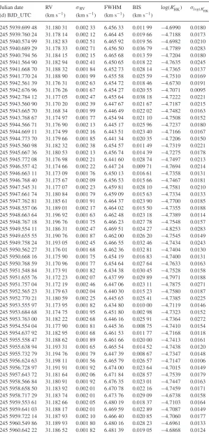
Table A1. HARPS 2012 data for CoRoT-7, processed in the same way as the 2008–2009 data (Queloz et al.2009). From left to right are given: Julian date, RV, the estimated errorσRVon

the RV, the FWHM and the line bisector of (BIS) of the cross-correlation function (as defined in Queloz et al.2001), the CaIIactivity indicator log(R_HK) and its errorσlog(R

HK).

Julian date RV σRV FWHM BIS log(RHK ) σlog(R_HK)

(d) BJD_UTC (km s−1₎ _{(km s}−1₎ _{(km s}−1₎ _{(km s}−1₎

245 5939.699 48 31.180 31 0.002 33 6.456 33 0.011 99 −4.6990 0.0180 245 5939.760 24 31.178 14 0.002 12 6.464 45 0.019 66 −4.7188 0.0173 245 5940.574 99 31.182 83 0.002 51 6.465 92 0.019 56 −4.6982 0.0210 245 5940.689 29 31.178 33 0.002 71 6.456 50 0.036 79 −4.7789 0.0283 245 5940.794 56 31.184 15 0.002 15 6.465 68 0.013 59 −4.7204 0.0180 245 5941.564 90 31.182 94 0.002 41 6.450 65 0.018 22 −4.7635 0.0245 245 5941.668 70 31.188 32 0.001 84 6.452 73 0.028 14 −4.7365 0.0137 245 5941.770 24 31.188 90 0.001 99 6.455 58 0.025 59 −4.7510 0.0169 245 5942.561 39 31.176 31 0.002 63 6.454 72 0.018 46 −4.6730 0.0191 245 5942.676 96 31.176 26 0.001 67 6.454 27 0.020 55 −4.7071 0.0095 245 5942.784 12 31.177 05 0.002 47 6.455 64 0.038 18 −4.7222 0.0221 245 5943.560 90 31.170 20 0.002 39 6.447 67 0.021 67 −4.7187 0.0215 245 5943.665 70 31.168 34 0.001 99 6.446 49 0.022 02 −4.7482 0.0163 245 5943.768 67 31.174 97 0.001 77 6.454 94 0.021 10 −4.7508 0.0152 245 5944.566 71 31.176 90 0.002 13 6.445 17 0.025 96 −4.7237 0.0180 245 5944.669 11 31.174 99 0.002 16 6.443 51 0.023 40 −4.7166 0.0167 245 5944.773 70 31.179 66 0.001 85 6.441 34 0.020 35 −4.7206 0.0150 245 5945.560 98 31.182 32 0.002 38 6.454 57 0.011 49 −4.7319 0.0221 245 5945.667 36 31.180 53 0.002 13 6.456 74 0.014 39 −4.7275 0.0178 245 5945.772 08 31.176 98 0.002 21 6.441 60 0.028 74 −4.7497 0.0213 245 5946.557 42 31.174 66 0.002 22 6.447 24 0.009 71 −4.7694 0.0214 245 5946.663 11 31.173 09 0.001 76 6.450 13 0.016 61 −4.7358 0.0131 245 5946.768 40 31.175 67 0.002 09 6.456 53 0.015 66 −4.7467 0.0181 245 5947.545 31 31.177 07 0.002 23 6.459 81 0.028 10 −4.7581 0.0210 245 5947.661 74 31.180 84 0.001 79 6.459 09 0.015 63 −4.7334 0.0133 245 5947.762 81 31.185 61 0.001 91 6.464 37 0.023 90 −4.7700 0.0185 245 5948.557 06 31.189 01 0.002 17 6.464 02 0.015 50 −4.7355 0.0188 245 5948.663 64 31.196 92 0.001 63 6.462 48 0.023 18 −4.7389 0.0114 245 5948.767 18 31.196 76 0.001 75 6.466 23 0.027 78 −4.7548 0.0157 245 5949.554 11 31.186 31 0.002 47 6.469 51 0.024 27 −4.8253 0.0283 245 5949.655 55 31.190 76 0.001 87 6.462 00 0.026 20 −4.7545 0.0149 245 5949.758 24 31.193 05 0.002 45 6.466 55 0.032 46 −4.7434 0.0243 245 5950.562 27 31.176 01 0.001 68 6.462 36 0.032 81 −4.7404 0.0130 245 5950.668 16 31.175 90 0.001 75 6.454 19 0.016 83 −4.7400 0.0131 245 5950.768 59 31.170 96 0.001 77 6.454 64 0.027 64 −4.7633 0.0163 245 5951.548 84 31.173 91 0.001 82 6.434 38 0.030 45 −4.7528 0.0158 245 5951.655 76 31.172 23 0.002 07 6.437 99 0.029 89 −4.7971 0.0188 245 5951.757 04 31.172 19 0.002 46 6.447 06 0.023 11 −4.7875 0.0271 245 5952.565 23 31.179 63 0.002 04 6.440 30 0.015 23 −4.7580 0.0187 245 5952.770 21 31.180 59 0.002 25 6.445 65 0.025 41 −4.7385 0.0225 245 5953.555 97 31.173 95 0.001 82 6.434 80 0.010 00 −4.7119 0.0146 245 5953.684 68 31.174 75 0.001 95 6.451 80 0.002 98 −4.7323 0.0152 245 5953.763 00 31.182 22 0.002 68 6.446 16 0.025 91 −4.7364 0.0272 245 5954.554 04 31.177 90 0.001 81 6.445 36 0.008 75 −4.7410 0.0154 245 5954.637 92 31.182 95 0.001 68 6.461 53 0.011 77 −4.7168 0.0118 245 5955.558 47 31.188 62 0.001 89 6.461 66 0.020 00 −4.7413 0.0161 245 5955.638 94 31.193 31 0.001 65 6.465 54 0.014 52 −4.7438 0.0120 245 5955.732 79 31.194 76 0.001 79 6.447 39 0.008 67 −4.7347 0.0148 245 5956.624 63 31.198 11 0.001 56 6.465 79 0.026 57 −4.7147 0.0106 245 5956.728 97 31.191 91 0.001 92 6.474 00 0.023 64 −4.7015 0.0149 245 5957.643 72 31.181 64 0.002 06 6.471 84 0.028 57 −4.7539 0.0179 245 5958.566 84 31.180 91 0.001 92 6.476 35 0.023 01 −4.7447 0.0163 245 5958.658 50 31.183 92 0.002 01 6.470 78 0.022 16 −4.7459 0.0171 245 5958.717 29 31.183 74 0.002 01 6.473 76 0.029 09 −4.6738 0.0158 245 5959.553 61 31.182 66 0.002 05 6.480 19 0.018 37 −4.7103 0.0164 245 5959.641 03 31.188 17 0.002 01 6.469 59 0.022 89 −4.7087 0.0149 245 5959.722 14 31.187 93 0.002 10 6.466 40 0.020 85 −4.7060 0.0177 245 5960.549 86 31.189 93 0.001 80 6.480 16 0.028 23 −4.6961 0.0133 245 5960.642 22 31.186 52 0.001 82 6.481 39 0.019 05 −4.6868 0.0124

(15)

[image:15.595.146.448.71.229.2]

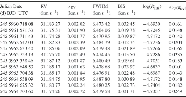
Table A1 –continued

Julian Date RV σRV FWHM BIS log(RHK ) σlog(R

HK)

(d) BJD_UTC (km s−1₎ _{(km s}−1₎ _{(km s}−1₎ _{(km s}−1₎

245 5960.718 08 31.183 27 0.002 02 6.473 42 0.032 45 −4.6930 0.0161 245 5961.571 33 31.175 31 0.001 90 6.464 06 0.019 78 −4.7245 0.0148 245 5961.711 43 31.174 28 0.001 77 6.470 95 0.019 87 −4.7172 0.0140 245 5962.542 03 31.182 83 0.002 39 6.484 79 0.012 74 −4.7236 0.0204 245 5962.633 40 31.186 06 0.002 09 6.479 48 0.021 89 −4.7266 0.0166 245 5962.723 13 31.175 70 0.002 49 6.474 45 0.015 50 −4.7286 0.0235 245 5963.558 46 31.187 12 0.001 87 6.480 49 0.019 61 −4.7051 0.0135 245 5963.648 53 31.185 17 0.001 63 6.478 68 0.023 97 −4.6832 0.0101 245 5963.704 38 31.185 17 0.001 84 6.476 91 0.022 48 −4.6987 0.0143 245 5964.558 09 31.184 75 0.001 95 6.487 80 0.030 89 −4.7172 0.0148 245 5964.625 32 31.180 77 0.002 24 6.480 25 0.022 73 −4.7404 0.0182 245 5964.703 60 31.174 26 0.002 72 6.479 58 0.031 71 −4.7357 0.0249

This paper has been typeset from a TEX/LA_{TEX file prepared by the author.}