Munich Personal RePEc Archive
Diversification in Crude Oil and Other
Commodities: A Comparative Analysis
Abdullah, Ahmad Monir and Saiti, Buerhan and Masih,
Abul Mansur M.
University of Kuala Lumpur, Malaysia, INCEIF
29 June 2014
Online at
https://mpra.ub.uni-muenchen.de/56988/
Diversification in Crude Oil and Other Commodities:
A Comparative Analysis
Ahmad Monir Abdullah
1*Buerhan Saiti
1Abul Mansur Mohammed Masih
21
UNIKL Business School, Yayasan Selangor Building,
Kampung Baru, 50300 Kuala Lumpur Malaysia
2INCEIF, Lorong Universiti A, 59100, Kuala Lumpur Malaysia
*Corresponding Author: [email protected]
Abstract:
An understanding of how volatilities of and correlations between commodity returns change over time including their directions (positive or negative) and size (stronger or weaker) is of crucial importance for both the domestic and international investors with a view to diversifying their portfolios for hedging against unforeseen risks. This paper is a humble attempt to add value to the existing literature by empirically testing the ‘time-varying’ and ‘scale dependent’ volatilities of and correlations of the sample commodities. Particularly, by incorporating scale dependence, it is able to identify unique portfolio diversification opportunities for different set of investors bearing different investment horizons or holding periods. In order to address the research objectives, we have applied the vector error-correction test and several recently introduced econometric techniques such as the Maximum Overlap Discrete Wavelet Transform (MODWT), Continuous Wavelet Transform (CWT) and Multivariate GARCH – Dynamic Conditional Correlation. The data used in this paper is the daily data of seven commodities (crude oil, gas, gold, silver, copper, soybean and corn) prices from 1 January 2007 until 31 December 2013. Our findings tend to suggest that there is a theoretical relationship between the sample commodities (as evidenced in the cointegration tests) and that the oil, gold and corn variables are leading the other commodities (as evidenced in the Vector Error-Correction models). Consistent with these results, our analysis based on the application of the recent wavelet technique MODWT tends to indicate that the gold price return is leading the other commodities. From the point of view of portfolio diversification benefits based on the extent of dynamic correlations between variables, our results tend to suggest that an investor should be aware that the gas price return is less correlated with the crude oil in the short run (as evidenced in the continuous wavelet transform analysis), but due to its high volatility, it offsets its benefit of diversification in the long run and that an investor holding the crude oil can gain by including corn in his/her portfolio (as evidenced in the Dynamic conditional correlations analysis). Our analysis based on the recent applications of the wavelet decompositions and the dynamic conditional correlations helps us unveil the portfolio diversification opportunities for the investors with heterogeneous investment horizons or holding stocks over different periods.
1. Introduction
Crude oil prices have remained low during the 1980s until 2000 with an average price of US$20 per barrel. From 2004 onward, the crude oil price has increased significantly with an increase from US$31 per barrel in 2004 to US$140 per barrel in 2008. By year 2013 the crude oil price has remained within the range of US$100 – US$110 as depicted in Chart 1. The demand for crude oil remain strong especially by emerging economies such as China and India and with the capacity constraints on the supply side, oil prices is expected to remain within US$100 per barrel for time being. Crude oil price changes affect almost all sectors of economies. It affects the prices of other commodities from the supply side and also the demand side. On the supply side, crude oil enters the aggregate production function of commodities through the usage of various energy-intensive inputs such as fuel for agricultural machine and transportation of the commodities. On the demand side, some commodities which are generated from crude oil such as synthetic rubber are used as a competing product. Gas and coal prices are also affected due to its substitutability with crude oil as sources of energy. The disposable incomes of oil exporting countries also increase with the increase in the oil price. Therefore, demand for certain commodities such as gold will increase with the increase in crude oil price.
Due to the important of crude oil commodity, therefore, the changes in the crude oil price will give significant impact to other commodities. Investors in commodities market would like to know the correlation of other commodities with crude oil for their diversification benefit.
The objective of this paper is to examine the causal relationship between crude oil price and other commodities (gas, gold, silver, copper, soybean and corn). We would like to find out the lead-lag relationship between the seven commodities under review and to identify whether cointegration exist among those variables. We also would like to find any diversification benefits of the commodities.
The unique contribution of the paper, among others, which enhances the existing literature is in
empirically testing for the ‘time-varying’ and ‘scale dependent’ volatilities of and correlations between the sample variables. Particularly, by incorporating the scale dependence, the paper is able to identify unique portfolio diversification opportunities for different set of investors bearing different investment horizons or stock-holding periods. Hence, the specific research questions of this study are as follows:
i. Does the cointegration exist between the crude oil price and the other commodities such as gas, gold, silver, copper, soybean and corn?
ii. Does the crude oil price cause the prices of the other commodities to increase/decrease in which past values of crude oil price able to improve the prediction of other commodities such as gas, gold, silver, copper, soybean and corn?
iii. Among the exogenous variables, which one is more exogenous at different time scale? iv. Which commodities should an investor invest in along with the crude oil commodity in order
to gain portfolio diversification benefits?
v. How would the portfolio diversification benefits change given different investor’s investment
horizons or stock-holding periods?
The results from each of the research questions are expected to have significant implications for investors in their decisions concerning portfolio allocations and investment horizons. In a summary, using recent data and modern empirical methodologies, this paper humbly attempts to fulfil the strategic information needs of investors intending to diversify their portfolios in commodities market across the world.
Chart 1: Crude Oil Price and Other Commodities
2. Literature Review
Many researchers have studied the impact of crude oil price on other commodities. Among the earliest study on the price co-movement is a research done by Pindyck and Rotemberg (1990) that introduce the excess co-movement hypothesis (ECH) between commodity prices. They argue that due to herd behaviour in financial markets, prices tend to move together. Pindyck and Rotemberg found that price of largely unrelated raw commodities have a persistence tendency to move together. Further study by Baffes (2007) estimates the degree of pass-through of crude oil price changes to the prices of 35 other internationally-traded primary commodities. The results indicated that the elasticity for the non-energy commodity index was estimated at 0.16 and the fertilizer index displayed the largest pass-through, followed by the index for food commodities. The implications of this finding is that if crude oil prices remain high, the recent commodities price increase are likely to last longer than previous boom cycle, especially for the food commodities, fertilizers, and precious metals (Baffes 2007). Saghaian (2010) investigated on the correlation between oil and commodity prices. The results of this study showed that there is a strong correlation among oil and commodity prices, but the evidence for a causal link from oil to commodity prices is mixed (Saghaian 2010).
Study on the co-movement between crude oil price and a series of agricultural commodities and gold has been done by Natanelov, Alam et al. (2011). A comparative framework is applied to identify changes in relationships through time and various cointegration methodologies and causality tests are employed. Results indicate that co-movement is a dynamic concept and that some economic and policy development may change the relationship between commodities. They also find that biofuel policy buffers the co-movement of crude oil and corn futures until the crude oil prices surpass a certain threshold (Natanelov, Alam et al. 2011).
Tang and Xiong (2010) investigate on the investment in the commodities index and find that futures prices of different commodities in the United States became increasingly correlated with crude oil prices. Their finding reflects a financialization process of commodities markets and this finding clarify the reason of huge appreciation in the price volatility of non-energy commodities in 2008 (Tang and Xiong 2010).
Research on the impact of crude oil is not only with other commodities but also with stock market variables, exchange rate and macroeconomic variables. Jammazi and Aloui (2010) research on the impact of crude oil price on stock market and find that the stock market variables respond negatively and temporarily to the crude oil changes during moderate (France) and expansion (UK and France) phases but not at level to plunge them into a recession phase. However, the effect of West Texas Intermediate
0 20 40 60 80 100 120 140 160
01-Jan-97 03-Apr- 01 04-Jul- 05 02-Oct- 09 31-De c- 13
(WTI) changes occurred in the expansion period has driven the Japanese stock market into a recession phase. This illustrate the important role that policy makers has to play in order to counteract any
inflationary impact of higher prices with monetary policy such as in UK and France. This is in contrary to policy maker in Japan, who may be unable to completely offset the increased variability of oil shocks which has contributed into the vulnerability of the stock market in Japan (Jammazi and Aloui 2010).
Vacha and Barunik (2012) investigated on the co-movement of the energy market by researching the interconnections between the main components of the energy sector in the time-frequency space. They find that some energy pairs show strong dynamics in co-movement in time during various investment horizons. The results suggest that when looking at the dependence of energy markets, one should always keep in mind its time-varying nature and look at it for various investment horizons. While the strongest dependence occurs during the periods of sharp price drops, it seems that the periods of recession creating fear in the markets imply a much higher downside risk to a portfolio based on these commodities. This inefficiency of the energy market is muted after recovery from the recession. They also find that the three commodities, heating oil, gasoline and crude oil strongly co-move, thus for the manager willing to keep a well-diversified portfolio, the trio will imply great exposure to risk. On the other hand, natural gas seems to be unrelated to all three commodities for all investment horizons as well as the studied time periods (Vacha and Barunik 2012).
In a summary, the literature studying crude oil price and its resulting impact for portfolio diversification strategies for commodities is limited and inconclusive with results reporting contradicting evidence. Hence this subject needs further investigation.
3. Theoretical Background
Two theories have been identified for this study. The first theory is by Pindyck and Rotemberg (1990) that introduce the excess co-movement hypothesis (ECH) between commodity prices, arguing that due to herd behaviour in financial markets prices tend to move together. They find that price of largely unrelated raw commodities have a persistence tendency to move together.
The second theory is by Markowitz on portfolio diversification theory. Markowitz shaped the modern portfolio theory where the volatility of a portfolio is less than the weighted average of the volatilities of the securities it contains given that the portfolio consists of assets that are not perfectly correlated in returns. The variance of the expected return on a portfolio can be calculated as:
σp2 = (ΣWi2σi2+ ΣΣWiWjCovij)
Where the sums are over all the securities in the portfolio, Wi is the proportion of the portfolio in security i,
σi is the standard deviation of expected returns of security i, and Covij is the covariance of expected
returns of securities of i and j. Assuming that the covariance is less than one (invariably true), this will be less than the weighted average of the standard deviation of the expected returns of the securities. This is why diversification reduces risk (Markowitz 1959).
4. Methodology
4. 1 Data
The data used in this paper is the daily data of seven commodities (crude oil, gas, gold, silver, copper, soybean and corn) prices from 1 January 2007 until 31 December 2013 and obtained from DataStream at INCEIF(International Centre for Education in Islamic Finance).
4.2 Time Series Techniques
This study employs a time series technique namely cointegration and error correction modeling in order to find empirical evidence of the nature of relations between crude oil price and other commodities. Standard time-series approaches has been adopted to test the hypothesis whether crude oil price leads (or lags) the other commodities under review. The recent time series studies based on cointegration have applied either vector error correction and/or variance decomposition methods for testing Granger causality or lead-lag relationship. We would apply the following standard procedures to test the lead-lag relationship: We will examine the unit-root tests and the order of the VAR, and then we will apply Johansen cointegration test. However, the evidence of cointegration cannot tell us which variable is leading and lagging. Therefore, we have to test through vector error correction model (VECM) that can indicate the direction of Granger causality both in the short and long run (Masih, Al-Elg et al. 2008). The VECM, however, cannot tell us which variable is relatively more exogenous or endogenous. The appropriate technique to identify the most exogenous and endogenous variable is variance decomposition technique. However, the software that we use to test the time-series techniques is limited to 150 observations for testing variance decomposition. Our daily data consist of 4,429 observations. Therefore, the 150 observations only produce a result that covers 5 month observation of our total data which is insufficient to give a reliable opinion. Therefore, we apply Maximum Overlap Discrete Wavelet Transformation (MODWT) to test the lead and lag of the identified exogenous variables in different time scale.
4.3 Maximum Overlap Discrete Wavelet Transformation (MODWT)
According to literature, both Discrete Wavelet Transform (DWT) and Maximal Overlap Discrete Wavelet Transform (MODWT) can decompose the sample variance of a time series on a scale-by-scale basis via its squared wavelet coefficients. However, the MODWT-based estimator has been shown to be superior to the DWT-based estimator (Percival 1995; Gallegati 2008). Therefore, we are going to apply Maximal Overlap Discrete Wavelet Transform (MODWT) in our study.
Whitcher et al. (1999, 2000) extended the notion of wavelet variance for the maximal overlap DWT (MODWT) and introduced the definition of wavelet covariance and wavelet correlation between the two processes, along with their estimators and approximate confidence intervals. To determine the magnitude of the association between two series of observations X and Y on a scale-by-scale basis the notion of wavelet covariance has to be used. Following Gençay et al. (2001) and Gallegati (2008) the wavelet covariance at wavelet scale j may be defined as the covariance between scale j wavelet coefficients of X and Y, that is ̃ ̃ .
An unbiased estimator of the wavelet covariance using maximal overlap discrete wavelet transform (MODWT) may be given by the following equation after removing all wavelet coefficients affected by boundary conditions (Gallegati 2008),
̃ ̃ ∑ ̃ ̃
̃ ̃ ̃ ̃
The wavelet cross-correlation coefficients ̃ , similar to other usual unconditional cross-correlation coefficients, are between 0 and 1 and offers the lead/lag relationships between the two processes on a scale-by-scale basis.
Starting from spectrum of scale j wavelet coefficients, it is possible to determine the asymptotic variance Vj of the MODWT-based estimator of the wavelet variance (covariance). After that,
we construct a random interval which forms a 100(1 − 2p)% confidence interval. The formulas for an approximate 100(1 − 2p)% confidence intervals MODWT estimator robust to non-Gaussianity for ̃ are provided in Gençay et al. (2002) and Gallegati (2008). According to empirical evidence from the wavelet variance, it suggests that Nj = 128 is a large enough number of wavelet coefficients for the large sample theory to be a good approximation (Whitcher, Guttorp et al. 2000; Gallegati 2008).
4.4 Multivariate GARCH – Dynamic Conditional Correlation
We relied on the Multivariate Generalised Autoregressive Conditional Heteroscedastic (MGARCH) model in Pesaran and Pesaran (2010). We tested for both normal and t distributions, to determine which would model our case at optimum level. Results of unconditional correlation coefficients could suffice to provide empirical evidence to answer our fourth research question. However, we require the computation of conditional cross-asset correlations in order to address the fourth objective in more comprehensive through using DCC-MGARCH computation as
̃ ( )
√
Where qij,t-1 are given by
̅ ( ) ̃ ̃
In the above, ̅ is the (i,j)th unconditional correlation, 1 and 2 are parameters such that 1 + 2 < 1,
and ̃ are the standardized asset returns.
We also test whether the computed volatility is mean-reverting by estimating (1 –λi1–λi2). Some
diagnostic tests are conducted to substantiate the validity of our models. For more detail regarding this model, it can be found in Pesaran and Pesaran (2010).
4.4 Continuous Wavelet Transformation (CWT)
To answer the fifth objective of our research, we need to apply continuous wavelet transform (CWT). A number of authors have recently started to use the continuous wavelet transform (CWT) in economics and finance research for example Saiti (2012). The CWT maps the original time series, which is a function of just one variable time-separate into function of two different variables such as time and frequency. One major benefit CWT has over DWT/MODWT is that we need not define the number of wavelets (time-scales) in CWT which generates itself according to the length of data. Other than that, the CWT maps the series correlations in a two-dimensional figure that allows us to easily identify and interpret patterns or hidden information (Saiti 2012). For both MODWT and CWT, we use the Daubechies (1992) least asymmetric wavelet filter of length L=8 denoted by LA (8) based on eight non-zero coefficients (Daubechies 1992). Previous studies on high-frequency data have shown that a moderate-length filter such as L = 8 is adequate to deal with the characteristic features of time-series data (Gençay, Selçuk et al. 2001; Gençay, Selçuk et al. 2001; In and Kim 2013). In the literature, it is argued that an LA (8) filter generates more smooth wavelet coefficients than other filters such as Haar wavelet filter.
The continuous wavelet transform (CWT) is obtained by projecting a mother wavelet onto the
The position of the wavelet in the time domain is given by u, while its position in the frequency domain is given by s. Therefore, the wavelet transform, by mapping the original series into a function of u and s, gives us information simultaneously on time and frequency. We need to apply a bivariate framework which is called wavelet coherence to be able to study the interaction between two time series, how closely X and Y are related by a linear transformation. The wavelet coherence of two time series is defined as:
Where S is a smoothing operator, s is a wavelet scale, is the continuous wavelet transform of the
time series X, is the continuous wavelet transform of the time series Y, is a cross wavelet transform of the two time series X and Y (Madaleno and Pinho 2012). For further details, interested readers may refer to Gencay et al (2001; 2002) and In and Kim (2013).
5. Empirical Findings and Interpretations
5.1 Findings and Interpretations of Standard Time-Series Techniques
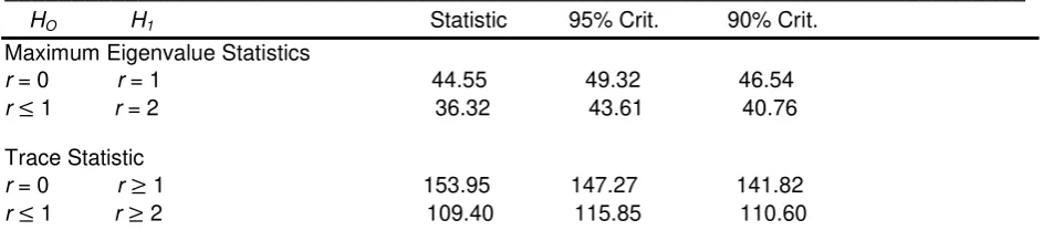
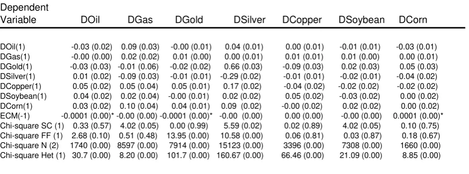
[image:8.595.70.542.661.770.2]We tested the unit roots of all the variables and found that they could be taken as I(1) on the basis of ADF tests. We also include wheat commodity in the beginning but we find it not I(1), therefore we have to drop wheat from our data. We also find that the optimal order of the VAR is two for AIC meanwhile for SBC, the optimal order of VAR is one. Therefore, we rely on AIC test by taking the optimal level of VAR as two. We applied the standard Johansen cointegration test (Table 1) and found them to have one cointegrating vector at 95% significance level on the basis of trace statistics. An evidence of cointegration implies that the relationship among the variables is not spurious and indicates that there is a theoretical relationship among the variables and they are in equilibrium in the long run. The cointegration test, however, cannot tell us the direction of Granger causality as to which variable is leading and which variable is lagging. We have applied the vector error correction modelling technique (Table 2) to identify the exogeneity and endogeneity of the variables. From Table 2, we can see that the crude oil, gold and corn variables are exogenous but the gas, silver, copper and soybean is endogenous. That tends to indicate that the gas, silver, copper and soybean variables would respond to the crude oil, gold and corn variables. The error correction model helps us distinguish between the short-term and long-term Granger causality. The error correction term stands for the long-term relations among the variables. The impact of each variable in the short term is given by the ‘F ’-test of the joint significance or insignificance of the lags of each of the ‘differenced’ variables. The diagnostics of all the equations of the error correction model (testing for the presence of autocorrelation, functional form and heteroskedasticity) tend to indicate that the equations are more or less well-specified.
Table 1: Johansen ML results for multiple cointegrating vectors of commodities
_____________________________________________________________________________
HO H1 Statistic 95% Crit. 90% Crit.
Maximum Eigenvalue Statistics
r = 0 r = 1 44.55 49.32 46.54
r 1 r = 2 36.32 43.61 40.76
Trace Statistic
r = 0 r 1 153.95 147.27 141.82
Table 2: Error correction model for seven commodities
_____________________________________________________________________________
Dependent
Variable DOil DGas DGold DSilver DCopper DSoybean DCorn
DOil(1) -0.03 (0.02) 0.09 (0.03) -0.00 (0.01) 0.04 (0.01) 0.00 (0.01) -0.01 (0.01) -0.03 (0.01)
DGas(1) -0.00 (0.00) 0.02 (0.02) 0.01 (0.00) 0.00 (0.01) 0.01 (0.01) 0.01 (0.00) 0.00 (0.01) DGold(1) -0.03 (0.03) -0.01 (0.06) -0.02 (0.02) 0.66 (0.03) -0.09 (0.03) 0.02 (0.03) 0.05 (0.03) DSilver(1) 0.01 (0.02) -0.09 (0.03) -0.01 (0.01) -0.29 (0.02) -0.01 (0.01) -0.02 (0.01) -0.04 (0.02) DCopper(1) 0.05 (0.02) 0.05 (0.04) 0.05 (0.01) 0.17 (0.02) -0.04 (0.02) -0.02 (0.02) -0.02 (0.02) DSoybean(1) 0.04 (0.02) 0.02 (0.04) -0.00 (0.01) 0.02 (0.02) 0.05 (0.02) -0.03 (0.02) 0.00 (0.02) DCorn(1) 0.03 (0.02) 0.10 (0.04) 0.04 (0.01) 0.09 (0.02) -0.00 (0.02) 0.02 (0.02) 0.00 (0.02) ECM(-1) -0.0001 (0.00)* -0.00 (0.00) -0.0001 (0.00)* -0.00 (0.00) 0.00 (0.00) -0.00 (0.00) 0.0001 (0.00)* Chi-square SC (1) 0.33 (0.57) 4.02 (0.05) 0.00 (0.99) 5.59 (0.02) 0.02 (0.89) 4.02 (0.05) 0.10 (0.75) Chi-square FF (1) 2.68 (0.10) 0.51 (0.48) 13.95 (0.00) 10.58 (0.00) 0.06 (0.81) 0.03 (0.87) 0.18 (0.67) Chi-square N (2) 1740 (0.00) 8597 (0.00) 7914 (0.00) 15123 (0.00) 3396 (0.00) 7308 (0.00) 1660 (0.00) Chi-square Het (1) 30.7 (0.00) 8.20 (0.00) 101.7 (0.00) 160.67 (0.00) 66.46 (0.00) 21.09 (0.00) 8.85 (0.00)
Notes: SEs are given in parenthesis. The diagnostics are chi-squared statistics for: serial correlation (SC), functional form (FF), normality (N) and heteroskedasticity (Het). The equations, therefore, are well specified.
* Indicate significance at the 5% level.
The proportion of the variance decomposition explained by its own past shocks can determine the relative exogeneity/endogeneity of a variable. However, the software that we use to test the variance decomposition limits our observations into 150 only whereby our total observation is 4,420. Therefore, in order to identify the lead-lag relationship between selected commodities, we apply Maximum Overlap Discrete Wavelet Transformation (MODWT).
5.2 Findings and Interpretations ofMaximum Overlap Discrete Wavelet Transformation (MODWT)
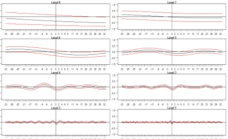
In Figure 1, we report the MODWT-based wavelet cross-correlation between the crude oil and gold at all period with the corresponding approximate confidence intervals, against time leads and lags for all scales, where each scale is associated with a particular time period. The individual cross-correlation functions correspond to – from bottom to top – wavelet scales …, which are associated with changes of 1-2, 2-4, 4-8, 8-16, 16-32, 32-64, 64-128 and 128-256 days. The red lines bound approximately 95% confidence interval for the wavelet cross-correlation. If the curve is significant on the right side of the graph, the second variable is leading. If the curve is significant on the left side of the graph, it is the opposite. If both the 95% confidence levels are above the horizontal axes, it is considered as significant positive wavelet cross-correlation; if both the 95% confidence levels are below the horizontal axes, it is considered as significant negative wavelet cross-correlation.
The Figure 1 indicates that the wavelet cross-correlation between crude oil and gold. From this figure, we could observe that:
i) At the wavelet levels of 1, 3, 4 and 5, we can observe that the graph skewed to the right which indicate that the gold price return leads the crude oil price return;
ii) At the wavelet level 6 which associated with 32-64 days, the graph skewed to left hand side with significant negative value which implies that the crude oil price return is leading the gold price return;
iv) Last but not least, at wavelet level 8 which associated with 128-256 days (around one year), more interestingly, we can observe that the there is significant negative wavelet cross-correlation on the right hand-side with implication of, again, the gold price return leads the crude oil price return.
We can conclude here that on the most of levels the gold price return leads crude oil price return. More importantly, there will be diversification benefit between these two commodities in the long-run.
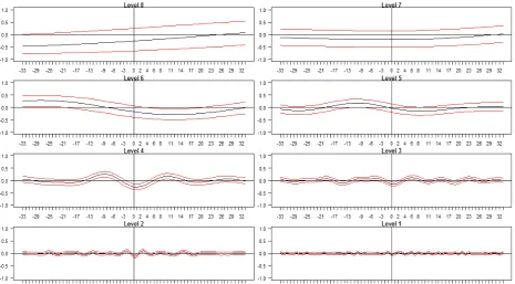
The Figure 2 shows that the wavelet cross-correlation between crude oil price return and corn price return. From this figure, we derive the following facts:
i) At the first wavelet level, we can observe that the graph skewed to the left which indicate that crude oil price return lead corn price return;
ii) At the wavelet level 7, there is no clear lead-lag relationship evidence between these two commodities;
iii) At other wavelet levels such as 2, 3, 4, 5, 6, and 8, we can observe that the graphs skewed to right hand-side with significant negative values. This implies that there is negative relationship between oil price return and corn price return. Is also may indicate that the corn price return is leading the crude oil price in the long-run.
Our results may suggest that the crude oil price return is leading in the short-term (1-2 days) and vice versa in the long-term.
The Figure 3 shows that the wavelet cross-correlation between gold price return and corn price return. From this figure, we may observe the followings:
i) At the wavelet levels 1 and 7, there is no clear lead-lag relationship evidence between these two commodities such as gold and corn price returns;
ii) From wavelet level 2 until wavelet level 6 (from 2-4 days until 32-64 days), the graphs skewed to right hand-side which implication of the leading role of corn price return. More importantly there is significant negative relationship between these two commodities.
iii) At level 8 which associated with 128-256 days (in the long-run), the graph skewed to left hand-side which significant negative value. This may imply that the gold price return leads corn price return.
We may conclude that, the corn price return leads the gold price return in the short-run and vice versa in the long-run. However, there would be diversification benefit between these two commodities, namely, gold and corn, in both short and long runs.
Figure 2: Maximum Overlap Discrete Wavelet Transformation:Crude Oil vs. Corn
[image:11.595.84.542.365.644.2]5.3 Findings and Interpretations of MGARCH-DCC
In order to assess the diversification benefits of the selected commodities, we have applied Dynamic Conational Correlation (MGARCH-DCC) instead of Constant Conational Correlation in this Section. Table 3 summarises the maximum likelihood estimates of and for the seven commodities prices returns, and and , comparing multivariate normal distribution with multivariate student t -distribution.
[image:12.595.75.541.71.328.2]The maximised log-likelihood value for the case of t-distribution [109,525.9] is larger than that obtained under the normality assumption [108,643.4]. The estimated degree of freedom for the t -distribution [8.5150] was below 30; and any other value one would expect for a multivariate normal distribution. This suggests that the t-distribution is more appropriate in capturing the fat-tailed nature of the distribution of price returns. Henceforth our analysis will work with the t-distribution estimates.
Table 4 shows the estimated unconditional volatilities (diagonal elements) and the unconditional correlations (off-diagonal elements) of the seven commodities prices. The numbers in parenthesis in the diagonal elements represent ranking of unconditional volatility (from highest to lowest). The ranking is characteristic of the volatility of the 7 commodities. The gas, crude oil and silver tend to receive a larger share of speculative trades in the commodities prices. Gold show the lowest volatility, reflecting the role of the gold as the best hedge instrument against inflation (Worthington and Pahlavani 2007).
More relevant to the fourth objectives of this paper are the correlations among the prices. A brief examination of the unconditional correlations reported in Table 4 highlight the fact that the gas price has the lowest correlations with other prices. To have a clearer picture of the relative correlation among prices, we ranked the unconditional correlations (from highest to lowest) as shown in Table 5.
Table 3: Estimates of and , and and , for the eight prices.
_____________________________________________________________________________
Multivariate normal Multivariate t
distribution distribution ___________________ _________________
[image:12.595.70.538.691.746.2]Lambda 1
(
)
Oil
.95511 184.2915
.95906 188.7528
Gas
.89181 114.2868 .88358 87.2526
Gold
.92761 118.4523
.94469 148.1534
Silver
.92634 104.5338
.94554 124.1494
Copper
.94380 145.9686
.94354 135.0838
Soybean
.91781 99.2804
.93300 108.4459
Corn
.93514 140.1689
.92901 106.8266
Lambda 2
(
)
Oil
.04201 9.3077 .03759 8.6517
Gas
.09658 15.0316 .10048 12.5046
Gold
.04799 10.3281 .04046 9.2763
Silver
.06125
9.5808 .04826 7.9035
Copper
.04666 9.9061 .04546 8.9818
Soybean
.05968 10.2666 .04786 8.8487
Corn
.04433 11.0828 .04695 9.1577
Delta 1
(
)
.99262 1031.1 .99140 814.9476
Delta 2
(
)
.00478 10.7114 .00547 9.7134
Maximised log-likelihood
108,643.4
109,525.9
Degree of freedom (df)
-
8.5150
[image:13.595.73.541.405.553.2]Note: and are decay factors for variance and covariance, respectively.
Table 4: Estimated unconditional volatility matrix for the 7 commodity prices
_____________________________________________________________________________
Oil Gas Gold Silver Copper Soybean Corn
Oil
.00953(2) .118400 .19187 .14250 .26477 .15241 .14016
Gas
.11840 .017298(1) .05877 .08592 .03084 .04172 .04821
Gold .19187 .058777 .00482(7) .44735 .30108 .11030 .10747
Silver .14250 .085925 .44735 .00914(3) .17149 .06909 .08191
Copper .26477 .030839 .30108 .17149 .00746(5) .20590 .18166
[image:13.595.70.544.608.766.2]Soybean
.
15241 .041723 .11030 .06909 .20590 .00716(6) .56035
Corn .14016 .048205 .10747 .08191 .18166 .56035 .00833(4)
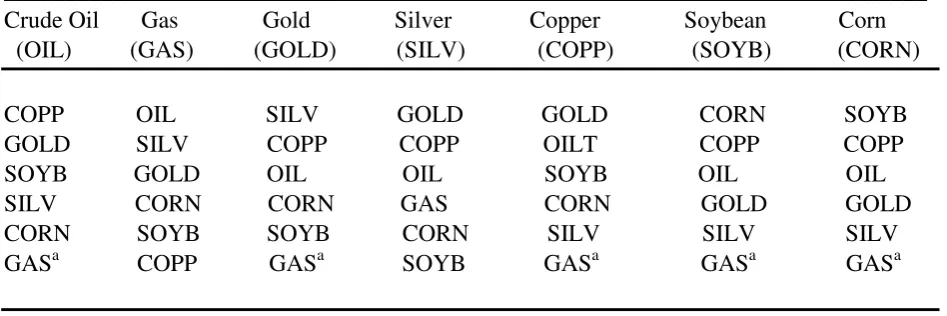
Table 5: Ranking of unconditional correlations among 7 commodities prices
_____________________________________________________________________________
Crude Oil Gas Gold Silver Copper Soybean Corn
(OIL) (GAS) (GOLD) (SILV) (COPP) (SOYB) (CORN)
COPP OIL SILV GOLD GOLD
CORN SOYB
The above rankings inform us two important facts. First, for almost all commodities (with the exception of silver), the lowest correlation is with the gas commodity (see notation ‘a’ in Table 5). This implies that in order to fully benefit from portfolio diversification, portfolio should include gas commodity. However, gas prices are the most volatile among all commodities. Therefore, investors will be exposed to higher risk due to higher volatility in gas price. Second and more pertinent, crude oil has the lowest correlation with gas, corn and silver. Therefore, based on unconditional result in Table 5, any investor with an exposure in crude oil and want to obtain maximum diversification with lowest risk should invest in gas commodity because gas has the lowest correlation with crude oil. Similar result is obtained for investors that has exposure in gold, copper, soybean and corn which indicate that they should hold gas commodity to obtain the maximum diversification benefit.
Thus far, our analyses and conclusions on volatilities and correlations have been made on unconditional basis. Unconditional basis mean we take the average volatility and correlation in the sample period. However, the assumption that volatility and correlation remain constant throughout a period spanning over 17 years does not appeal to intuition. It is more likely that volatility and correlation are dynamic in nature and it is this aspect which the Dynamic Correlation Coefficient (DCC) model employed in this paper addresses.
We start with observing the temporal dimension of volatility. We chart the conditional volatilities for the seven commodities prices as per Chart 2 below. During those 17 years under observation, we noticed that gas commodity prices has the highest volatility compare to others. The lowest volatility during that period is gold commodity. During the period of the Southeast Asian Financial Crisis of 1997/98, crude oil price significantly increase in volatility meanwhile gold remain constant. . The highest increase in volatility for crude oil price and other commodities (with the exception of gas) are during the Global Financial Crisis in 2008 as illustrated in Chart 2 and 3. We also noticed that the volatility for almost all commodities during Global Financial Crisis in 2008 is higher than the volatility during Asian Financial Crisis in 1997/1998. Gas price is extremely volatile compare against other commodities and it randomly volatile throughout those 17 years under observation. From the chart below, we can conclude that it is very risky to invest in gas commodity since it is highly volatile and unpredictable compare against other commodities. We also notice that gold is the lowest volatile commodity compare to the rest of commodities as illustrated in Chart 2 and 3.
Chart 2: Conditional Volatilities of All Commodities
Chart 3: Conditional Volatilities of Crude Oil, Gold and Corn 0.00
0.01 0.02 0.03 0.04 0.05 0.06 0.07
29-Jan-97 24-Apr-01 18-Jul-05 09-Oct-09 31-De c-13 Plot of conditional volatilities
Vol(OIL) Vol(GAS ) Vol(GOLD) Vol(SILV ER)
Through conditional correlations as described in Chart 4 and 5 below, we compare the correlation between crude oil prices with other commodities. We noticed that from year 1997 until 2010, correlations of the crude oil with other commodities showing uptrend with huge increase during the Global Financial Crisis in 2008. From 2010 to 2013, the trend of correlation is downward due to correction after the huge shock in 2008. The highest correlation of crude oil is with copper and the lowest correlation of crude oil is with gas. The second lowest correlation of crude oil is with corn. Investor that having exposure portfolio in crude oil is better off with diversification in corn rather than gas because gas price volatility is too high which offset it benefit as a diversification commodity. Corn not only the second lowest correlation with crude oil but corn is also exogenous variable as identified in our previous test (please refer to Table 2).
Chart 4: Conditional Correlation of Crude Oil with Other Commodities
Chart 5: Conditional Correlation of Crude Oil with Corn, Silver & Gas
0.000 0.005 0.010 0.015 0.020 0.025
29-Jan-97 24-Apr-01 18-Jul-05 09-Oct-09 31-De c-13
Plot of conditional volatilities
Vol(OIL) Vol(GOLD) Vol(CORN)
-0.2 -0.1 0.0 0.1 0.2 0.3 0.4 0.5
29-Jan-97 24-Apr- 01 18-Jul- 05 09-Oct- 09 31-De c- 13
Plot of conditional correlations
5.4 Correlation of Commodities at different time and investment horizons based on the Continuous Wavelet Transform
Chart 6 to 11 present the estimated continuous wavelet transform and phase difference for commodities price from scale 1 (one day) up to scale of 9 (approximately two market years, 512 days). Time is shown on the horizontal axis in terms of number of trading days, while the vertical axis refers to the investment horizon. The curved line below shows the 5% significance level which is estimated using Monte Carlo simulations. The figure follows a colour code as illustrated on the right with power ranges from blue (low correlations) to red (high correlations).
Any investor that interested to hold crude oil commodity as his main portfolio, he will need to diversify his portfolio by having another commodity to gain diversification benefit. Gold is a good diversification portfolio for crude oil in low scale (high frequency) below 256 holding period or one year. From August 2006 onward, gold and crude oil highly correlate for long term investment horizon which is more than one year or 256 days (please refer to Chart 6). Therefore, investor who has an exposure in crude oil and intend to diversify his portfolio, he should not hold gold portfolio more than one year in order to get the benefit of diversification.
For investor that interested to hold portfolio of crude oil and corn, he should hold that investment for short period of time (within 1 day to 32 days) in order to obtain the diversification benefit. If his investment is beyond one years or more than 256 days, he also will be gain diversification benefit (please refer to Chart 7). From the Chart 7 also we noticed that during Global Financial Crisis in 2008, the correlation between crude oil and corn is very high for investment holding of 32- 256 days.
Soybean and crude oil correlation also has similar effect like corn and crude oil correlation where the short term investment horizon (within 1 to 32 days) will give better diversification benefit compare against high scale time horizon. From year 2008 onward, soybean price highly correlate with crude oil in the scale of 256 to 512 day (please refer to chart 8).
The correlation between crude oil and gas is low at lower scale (between 1 to 256 days). However, the correlation beyond 256 days or a year is very high. The arrow in the Chart 9 for hot area pointing to the left which indicate that the correlation between crude oil and gas is positively related.
Copper and crude oil correlation also only give diversification benefit in short term investment horizon (from 1 day to 32 days). If the investment horizon for crude oil with copper is within 64 until 128 days, the investor also will gain diversification benefit (please refer to chart 10). From the investment horizon of 256 days to 512 days, copper is highly correlate with crude oil from year 2004 until 2013. Before those years, the correlation between the two commodities is very low.
The correlation between crude oil and silver also quite similar with correlation between copper and crude oil. At the lower scale until 32 days, investor will gain diversification benefit. From 32 to 64 days investment horizon, the correlation is very high during Global Financial Crisis in 2008. If the investment horizon is within 64 until 128 days, the investor will also gain diversification benefit. Within the investment horizon of 256 days to 512 days, silver is highly correlate with crude oil from year 2004 until
-0.2 -0.1 0.0 0.1 0.2 0.3 0.4
29-Jan-97 24-Apr- 01 18-Jul- 05 09-Oct- 09 31-De c- 13
Plot of conditional correlations
2013. This phenomena is not seen before those years, where the correlation between the two commodities is very low.
[image:17.595.200.411.169.292.2]We can clearly see the contributions of the wavelet transformations in helping us understand portfolio diversification opportunities for investors with different investment horizons.
Table 6: Date for Horizontal Axis
Horizontal Axis Date
500 December 1998
1000 November 2000
1500 October 2002
2000 September 2004
2500 August 2006
3000 July 2008
3500 June 2010
4000 May 2012
Chart 6: Continuous Wavelet Transform – Gold vs. Crude Oil Chart 7: Continuous Wavelet Transform – Crude Oil vs. Corn
Chart 8: CWT – Crude Oil vs. Soybean Chart 9: CWT– Crude Oil vs. Gas
Chart 10: CWT – Crude Oil vs. Copper Chart 11: CWT – Crude Oil vs. Silver
P
e
ri
o
d
Gold vs. Crude Oil
500 1000 1500 2000 2500 3000 3500 4000 4 8 16 32 64 128 256 512 1024 0 0.1 0.2 0.3 0.4 0.5 0.6 0.7 0.8 0.9 1 P e ri o d
Crude Oil vs. Corn
500 1000 1500 2000 2500 3000 3500 4000 4 8 16 32 64 128 256 512 1024 0 0.1 0.2 0.3 0.4 0.5 0.6 0.7 0.8 0.9 1 P e ri o d
Crude Oil vs. Soybean
500 1000 1500 2000 2500 3000 3500 4000 4 8 16 32 64 128 256 512 1024 0 0.1 0.2 0.3 0.4 0.5 0.6 0.7 0.8 0.9 1 P e ri o d
Crude Oil vs. Gas
6. Concluding Remarks
Firstly, from the vector error-correction analysis, we conclude that the crude oil, gold and corn variables are exogenous but the gas, silver, copper and soybean are endogenous. That tends to indicate that the gas, silver, copper and soybean variables would respond to the crude oil, gold and corn variables.
Secondly, based on MODWT, we observe that: i) on the most of levels the gold price return leads crude oil price return. More importantly, there will be diversification benefit between these two commodities in the long-run; ii) the results of wavelet cross-correlation between crude oil and corn may suggest that the crude oil price return is leading the corn price return in the short-term (1-2 days) and vice versa in the long-term; iii) as far as gold price and corn are concerned, the corn price return leads the gold price return in the short-run and vice versa in the long-run. However, there would be diversification benefit between these two commodities, namely, gold and corn, in both short and long runs.
Thirdly, according to MGARCH-DCC, the results indicate that almost all commodities (with the exception of silver) have the lowest correlation with the gas commodity. The crude oil has the lowest correlation with gas, corn and silver. However, it is very risky to invest in gas commodity since it is highly volatile and unpredictable compared to other commodities.
Fourthly, the application of CWT indicate that short term investment horizon (within 32 days holding period) will generate portfolio diversification benefit for investors having exposure in crude oil and at the same time hold other commodities such as corn, soybean, copper and silver. For gold and gas portfolio against crude oil, the investor can gain diversification benefit if he/her hold his/her portfolio within one year or 256 days.
Last but not the least, investor having portfolio exposure in crude oil is better off with diversification in corn rather than gas because gas price volatility is too high which offsets its benefit as a diversification commodity. Corn has not only the second lowest correlation with crude oil but corn is also exogenous variable.
We can clearly see the contributions of the wavelet transformations in helping us understand portfolio diversification opportunities for investors with different investment horizons.
References
Baffes, J. (2007). "Oil spills on other commodities." Resources Policy
32
(3): 126-134.
Daubechies, I. (1992). Ten lectures on wavelets, SIAM.
P
e
ri
o
d
Crude Oil vs. Copper
500 1000 1500 2000 2500 3000 3500 4000 4 8 16 32 64 128 256 512 1024 0 0.1 0.2 0.3 0.4 0.5 0.6 0.7 0.8 0.9 1 P e ri o d
Crude Oil Vs. Silver