Proceedings
One day international research workshop on
Super-Toroidal
Electrodynamics
5 November 2004, University of Southampton
Edited by A.Boardman and N.Zheludev
EPSRC Adventure Fund Project
IOP Quantum Electronics and Photonics Group
Table of Contents
1.
List of Participants and Group Photo
2.
Workshop Timetable
3.
The Donut Game. Intriguing Properties of Super-Toroidal
Currents (by Nikolay Zheludev)
4.
Simplest Sources Of Electromagnetic Fields as a Tool for
Testing the Reciprocity-Like Theorems (by Georgii
Afanasiev)
5.
Topological Invariants in Molecular Networks, and Their
Current-Like Observables (by Aurnout Ceulemans)
6.
Toroidal Moments and Atomic Emission in Condensed
Media (by Eugene Tkalya)
7.
Toroidal Moments in Spin-Ordered Crystals (by Hans
Schmid)
8.
Toroidal Electrodynamics and Solid State Physics (by
Mikhail Martsenyuk)
List of Participants:
1. Dr. Carlos Vaz, Cambridge University, UK
2. Prof. Alain Dereux, University of Bourgogne, France 3. Dr. Martin McCall, Imperial College, UK
4. Prof. David Hanna, University of Southampton, UK
5. Prof. Arnout Ceulemans, Catholic University of Leuven, Belgium 6. Prof. Will Stewart, University of Southampton, UK
7. Prof. Mikhail Martsenyuk, Perm State University, Russia 8. Dr. Adrian Potts, University of Southampton, UK
9. Dr. Konstantin Vyatkin, Perm State University, Russia 10. Dr. Eugeny Tkalya, Moscow State University, Russia 11. Dr. Gerasim Galitonov, University of Southampton, UK 12. Prof. Hans Schmid, University of Geneva, Switzerland 13. Mr. Justin Llandro, Cambridge University, UK
14. Dr. Vassili Fedotov, University of Southampton, UK
15. Dr. Georgii Afanasiev, Dubna Joint Institute for Nuclear Research, Russia 16. Dr. Kiril Marinov, Salford University, UK
17. Dr. Thomas Moore, Cambridge University, UK 18. Dr. John Chad, University of Southampton, UK
19. Prof. Nikolay Zheludev, University of Southampton, UK 20. Mr. Tom Hayward, Cambridge University, UK
21. Mr. Alexandre Mary, University of Bourgogne, France
22. Prof. Allan Boardman, Salford University, UK (not present on the photo) 23. Mr. Sam Birtwell, University of Southampton, UK (not present on the photo) 24. Dr. Stephan Steinmuller, Cambridge University, UK (not present on the photo) 25. Dr. Kevin MacDonald, University of Southampton, UK (not present on the photo) 26. Mr. Desmond Tse, Cambridge University, UK (not present on the photo)
EPSRC Adventure Fund Project
IOP Quantum Electronics and Photonics Group
EPSRC NanoPhotonics Portfolio Centre, University of Southampton One day international research workshop on
Super-Toroidal Electrodynamics
5 November 2004, University of Southampton
Workshop Timetable
Duration of talks: 30 min + 10 min for discussion
9:00 Participants arrive, coffee
9:15 Welcoming message from IOP and EPSRC Adventure Fund Project by Allan Boardman and Nikolay Zheludev
Morning Session. Chair: Professor Nikolay Zheludev, University of Southampton
9:30 “Electromagnetic toroidal sources and their applications” by Georgii Afanasiev, Joint Institute for
Nuclear Research, Dubna, Russia
10:10 “Topological Invariants in Molecular networks, and their current-like observables” by Aurnout
Ceulemans, Catholic University of Leuven, Belgium
10:50 Coffee break
11:20 “Toroidal moments and atomic emission in condensed media” by Eugene Tkalya, Nuclear Research
Institute, Moscow state University, Russia
12:00 Lunch
Afternoon Session. Chair: Professor Will Stewart, University of Southampton
13:30 “Toroidal moments in spin-ordered crystals” by Hans Schmid, University of Geneva
14:10 “Toroidal electrodynamics and solid state physics” by Mikhail Martsenyuk, Perm State University,
Russia
14:50 Tea break
15:20 “From the detection of the magnetic component of optical near-fields to nano-torus plasmons carrying a magnetic dipole moment at optical frequencies” by Alain Dereux, University of Bourgogne, France.
Open discussion. Chair: Professor Allan Boardman, Salford University
THE DOUGHNUT GAME
Intriguing Propertied of Super-Toroidal Currents
(a brief literature review)
by N.Zheludev
THE DOUGHNUT GAME
Intriguing Propertied of Super-Toroidal Currents
(a brief literature review)
1 .
F ro m A C u rre n t L o o p to S u p e rto ro id a l C u rre n ts
2 .
E le c tro m a g n e tic R a d ia tio n o f S u p e rto ro id a l
C u rre n t
3 .
S u p e rto ro id a l C u rre n ts in E x te rn a l F ie lds
4 .
In te ra c tio n B e tw e e n S u pe rto ro id a l C u rre n ts
5 .
M o le c u la r T o ro id a l M o m e n ts
6 .
Ve c to r P o te n tia l o f S u p e rto ro id a l C u rre n ts a n d th e
A h a ro n o v -b o h m E ffe c t
A f a n a s i e v , 1 9 9 0 , 1 9 9 3 , 1 9 9 4 , 2 0 0 1
A f a n a s i e v & S t e p a n o v s k i, 1 9 9 5
A f a n a s i e v & D u b o v i k , 1 9 9 8
A h a r o n o v & B o h m , 1 9 5 9
C e u l e m a n s , C h i b o t r a u , F o w le s , 1 9 9 8
D u b o v ik , M a r t s e n y u k , S a h a , 2 0 0 0
D u b o v i k & T u g u s h e v , 1 9 9 0
F e i n b e r g , 1 9 6 3
H e a l d , 1 9 8 8
H e l w a r t h , N o u c h i, 1 9 9 6
J a k l e v ic h & o t h e r , 1 9 6 4
M a r t s e n y u k & M a r t s e n y u k , 1 9 9 1
M i l le r , 1 9 8 4
N e v e s s k i , 1 9 9 3
P a g e , 1 9 7 1
P o p o v , K a d o m t s e v a & o t h e r , 1 9 9 9
T o ls t o i & S p a r t a k o v , 1 9 9 0
T o n o m u r a , 1 9 9 5
V l a d , 1 9 9 5
Z e ld o v i c h , 1 9 5 7
Z h e l u d e v Iv a n , 1 9 7 6
A CURRENT LOOP
n
I
LJ
=
I
Ln
ϕδ ρ δ δ
(
−
)
( )
z
=
curl
M
d
R
L
I
d curl
r
<<
→
π
2
δ
3
(
n
( ) )
M
=
I
L
n
θ ρ δ δ
(
−
)
( )
z
d
R
L
I
d
r
<<
→
π
2
δ
3
n
( )
Current
Magnetization
The current loop is equivalent
to the magnetization of a sheet
enclosed by the loop
Ampere Law
POLOIDAL CURRENT ON A TORUS
J
M
The poloidal current on a torus
is equivalent to the magnetization
confined to the interior of the torus
J = curl M
M = curl T
( since div M = 0)
T
HIERARHY OF TOROIDAL CURRENTS
m=0
m=1
m=2
m=3
m=2
m=3
m=4
J
m
=
f
m
( )
t curl
(
m
+
1
)
(
n
δ
3
( ))
r
Current loop
J
0
=
f
0
( )
t curl
(
n
δ
3
( ))
r
3D Fractal
m=0
m=1
m=2
m=3
2D Fractal
SUPERTOROIDAL CURRENT AS A 3D FRACTAL
ELECTROMAGNETIC POTENTIALS
E
A
A
= −
−
=
1
c
t
grad
curl
∂
∂
Φ
H
A'
= + ∇
A
= −
f
c
f
t
Φ Φ
'
1
∂
∂
Scalar and Vector Potentials
ELECTROMAGNETIC FIELDS
OF SUPER-TOROIDAL SOLENOIDS
E
evenH
evenS
m = 2k
Supertoroidal
current
H
oddE
oddS
m = 2k+1
Supertoroidal
current
A
m
r
n
m
m
m
r
d
dt
D f
t
∝ ×
2
(
( ))
m = 2k, “magnetic” type super-currents
S
r
=
c
E
× ∝
H
r
4
2
2
π
θ
sin
The Pointing vector
“Magnetic” type super-current
“Electric” type super current
Vector-Potential of radiation
If a current oscillates in:
A current loop or super-toroidal coil of even order (m=2k)
= “magnetic” type radiation source
INTERACTION OF A CURRENT LOOP WITH
EXTERNAL FIELS
U
c
dV
c
dV
eraction
ext
ext
int
=
=
1
1
J A
M H
µ
=
I
π
d
c
L
2
n
n
I
Ld
ext
→
0
→
−
µ
INTEEERACTION OF SUPER-TOROIDAL CURRENTS
WITH EXTERNAL FIELDS
n
H
ext
,E
ext
U
f
t
t
t
m
m
m
int
( )
( )
∝
n
∂
H
ext
∂
U
f
t
t
t
m
m
m
int
( )
( )
∝
n
∂
E
ext
∂
m = 2k, “magnetic” type interaction
m = 2k+1, “electric” type interactions
m =o: current loop with H
m = 1, toroidal solenoid with current
Toroidal Solenoid and Electric Field
Zeldovich, 1957
Toroidal Solenoid immersed in electrolyte with current
Will be subjected to a moment of force
M
INTERACTION BETWEEN CURRENTS
n
1
J
1
n
2
J
2
A
2
A
1
E
c
dV
12
1
= −
J
1
(
r r A
−
1
)
2
(
r r
−
2
)
E
c
dV
21
2
1
= −
J
2
(
r r
−
)
A r r
1
(
−
1
)
E
int
=
E
12
+
E
21
E
12
=
E
21
INTERACTION BETWEEN
ODD- and EVEN-order TOROIDAL CURRENTS
Afanasiev, 2001
n
1
J
1
n
2
J
2
A
2
A
1
R
12
E
f
t
R
D f (t)
t
m
m
m
m
12
1
2
12
1
2 1
2
1
2 1
∝
( )
×
+
+
+
+
(
)
(
)
(
)
n (R
1
12
n )
2
∂
∂
Even type current: m
1
= 2q
Odd type current: m
2
= 2p+1
J
1
1
1 1
n
1
3
r r
1
=
f
t curl
m
+
−
( )
(
)
(
δ
(
))
J
2
=
f
2
( )
t curl
(
m
2 1
+
)
(
n
2
δ
3
(
r r
−
2
))
E
f
t
R
D f (t)
t
m
m
m
m
21
2
2
21
1
2 1
1
1
2 1
∝
( )
×
+
+
+
+
(
)
(
)
(
)
n (R
2
21
n )
1
∂
∂
VIOLATION OF ACTION-REACTION EQUILITY:
AN EXAMPLE
(G.N.Afanasiev, 2001)
No Fields are Generated by
a DC current outside toroid
Oscillating magnetic and electric fields
are generated by AC current in the loop
m = 0
m=1
E
t
f
t
LT
∝
T
=
∂
∂
3
3
( )
0
E
t
f
t
TL
∝
L
≠
∂
∂
3
The Reciprocity Relations
E
12
=
J E
1
2
dV
=
E
21
=
J E
2
1
dV
H
12
=
J H
1
2
dV
=
H
21
=
J H
2
1
dV
The Lorentz Lemma
The Feld-Tai Lemma
Maxwell’s equation for current 1
Maxwell’s equation for current 2
Some algebra
+ harmonic time dependencies
Limitations of the Reciprocity Relations
Afanasiev, 2001
If time dependent currents are involved the reciprocity relations are applicable if:
1.
The time dependencies are the same for all space points of a particular source
2.
The time dependencies in source 1 and source 2 are the same
E
12
=
J E
1
2
dV
=
E
21
=
J E
2
1
dV
H
12
=
J H
1
2
dV
=
H
21
=
J H
2
1
dV
The Lorentz Lemma
Reciprocity of Radio Transmission
V
U
R
R
transmitter
Free-space Communication line
Receiver
TOROIDAL POLARIZATION IN CONDENCED
MATTER PHYSICS
Dubovik, Martsenyuk, Saha, 2000
M
curl T
M
M
T
P
P
T
+
+
curl
curl
m
e
Magnetization and polarization
with account of toroidal moments:
j
total
j
P
M
t
c curl
= +
∂
+
∂
Total Current in Maxwell equations:
m
t
e
e
c
t
∂
∂
∂
∂
2
2
r
E
r
B
=
+
[
×
]
The equation of motion with toroidal force:
+
4
π
−
1
∂
×
∂
e curl
c
t
curl
(
T
e
[
r
T
m
])
+
∂
+
∂
curl
t
c curl curl
e
m
T
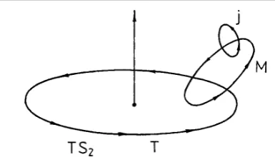
MOLECULAR MOMENTA
d
d
d
d
d
d
T
em
T
mm
m
m
m
m
r
r
d
m
Dipole
Magnetic Dipole
“Electric” toroidal moment
“Magnetic” toroidal moment
T
e
=
1
r
×
d
2
T
m
=
1
r
×
m
AROMAGNETISM
K
∝
- [ T x
∂
H/
∂
t ]
Oscillating Magnetic Field
Microcrystals of aromatic,
nonmagnetic substances
(antracene, pheantherene,
With benzene ring)
Show NO magnetism
of orbital or spin origin
Optical Detection of induced
birefringence
Tolstoi & Spartakov (1990)
Martsenyuk & Martsenyuk (1991)
H
H
H
H
H
H
O
O
CALCULATION OF MOLECULAR TOROIDAL
MOMENTA
H
H
H
H
H
H
O
O
O
Phloroglycine Molecule shows T
e
120 atoms Carbon Toroids show T
m
Current included by uniform magnetic field
DC CURRENT IN A TOROIDAL SOLENOID
Page (1971)
X
O
Vector
potential
Toroidal Solenoid
DC current:
a Toroidal Solenoid has NO external magnetic & Electric fields
but
THE AHARONOV-BOHM EFFECTS AND TOROIDAL
CURRENTS
Aharonov-Bohm, 1959
In QM vector potential cannot be illuminated
from the basis equations
Do Potential have independent significance
from the Fields?
ψ
ψ ψ
π
0
0
0
2
0
⇔
=
⇔
=
+
=
H
e
H
H
V
where
S
V t dt
i
S h
/
( )
H
e
c
m
=
[
P
−
A
]
2
2
THE AHARONOV-BOHM EFFECT
Aharonov & Bohm, 1959
Electron beam
Interference
Region
∆
φ
= −
2
π
e
d
= −
2
π
e
d
h
A s
h
B S
Phase shift
depends on the vector potential along the pass
(inconceivable in classical electrodynamics, no forces):
DC Toroidal Solenoid
Vector potential,
TONOMURA’s AHARONOV-BOHM EXPERIMENTS
first claim: Jaklevic, Lambe & other, 1964
PHOTOLITHOGRAPHICALLY
MANIFACTURED
MAGNETIZED TOROID
WITH SUPERCONDUCTION SHEELD
(prevents magnetic field to leak)
Trapped magnetic flux from 0 to 4h/e
ELECTRON INTERFERENCE
EXPERIMENT
TONOMURA’s EXPERIMENTS
ϕϕϕϕ
=0
No trapped field
ϕϕϕϕ
=
ππππ
NON-RADIATING CONFIGURATION: DC CURRENT
IN A TOROIDAL SOLENOID
and AN OSCILLATING ELECTRIC DIPOLE
Afanasiev, 2001
X
O
Vector potential Toroidal Solenoid
DC Excitation:
a Toroidal Solenoid has NO external
magnetic & Electric fields
Oscillating Dipole
U
c
dV
dipole
tor
dipole
tor
=
[
ρ
Φ
−
1
j
A
]
j
dipole
f
n
r
r
dipole
t
= −
∂
−
∂
δ
3
(
)
U
= −
1
n A
c
f
t
tor
∂
∂
Interaction Energy
FIELD-LESS SOURCES
OF OSCILLATING POTENTIALS???
(Afanasiev 2001)
H
oddE
oddS
m = 1
Toroidal
current
φ
=
0
A
= −
n
+
r (r .n)
c r
3
G t
( )
c r
3 3
F t
( )
E
= −
n
+
r (r .n)
c r
4
t
G t
c r
4 3
t
F t
∂
∂
( )
∂
∂
( )
H
= ×
r
n
c r
4 2
t
D t
2
2
∂
∂
( )
H
dipoleE
dipoleS
Oscillating Dipole
E
= −
n
+
r (r .n)
c r
4
t
G t
c r
4 3
t
F t
∂
∂
( )
∂
∂
( )
H
= ×
r
n
c r
4 2
t
D t
2
2
∂
∂
( )
φ
= −
(
n.r
)
( )
cr
2
D t
A
= −
n
c r
t
F t
∂
∂
( )
Electromagnetic Permutations in Free Space
:
(
∇ −
2
) ( , )
=
2
2
2
1
0
c
t
f
t
∂
∂
r
The Helmholtz wave equation
f
=
f z
1
(
−
ct
)
+
f
2
(
z
+
ct
)
Solution in the form of perturbations propagating with speed of light :
Flying Doughnuts
Hellwarth & Nouchi, 1996
Schematic of ”focused doughnut”
f
f
e
q
i
s q
s q
=
+
+
−
0
3
1
2
/
(
τ
)(
)
α
Ziolkowski (1989) discovered a class of generating
Functions which satisfies Helmholtz wave equations:
Here q
1,2 3
- parameters
S is a function of coordinates and
σ
τ
= z-ct;
σ
=z+ct
Vector Generalization
→
→
→
→
“Non-pathological” toroidal wave packets
which are neither transverse electric or transverse magnetic
A r
( , )
t
=
C curl
(
z
f
( , ))
r
t
Flying Doughnuts
Hellwarth & Nouchi, 1996
Schematic of ”focused doughnut”
J. Phys. D: Appl. Phys.34(2001) 539–559 www.iop.org/Journals/jd PII: S0022-3727(01)16545-9
Simplest sources of electromagnetic fields
as a tool for testing the reciprocity-like
theorems
G N Afanasiev
Bogoliubov Laboratory of Theoretical Physics, Joint Institute for Nuclear Research, Dubna, Moscow District 141980, Russia
E-mail: [email protected]
Received 22 August 2000, in final form 30 November 2000 Abstract
Electromagnetic fields of the simplest time-dependent sources (current loop, electric dipole, toroidal solenoid, etc), their interactions with an external electromagnetic field and between themselves are found. They are applied to the analysis of the Lorentz and Feld–Tai lemmas (or reciprocity-like theorems) having numerous applications in electrodynamics, optics, radiophysics, electronics, etc. It is demonstrated that these lemmas are valid for more general time dependences of the electromagnetic field sources than it was suggested up to now. It is shown also that the validity of
reciprocity-like theorems is intimately related to the equality of
electromagnetic action and reaction: both of them are fulfilled or violated under the same conditions. Conditions are stated under which
reciprocity-like theorems can be violated. A concrete example of their violation is presented.
1. Introduction
The reciprocity theorem has a long history in physics. It originates from the third Newtonian law stating equality of action and reaction. Later, Rayleigh, in the first volume of his encyclopaedic treatise ‘Theory of Sound’ [1] proved certain relations between the forces acting between two physical systems and the displacements induced by them. Since there is no time retardation in the Newtonian mechanics, this statement looks almost trivial. Furthermore, Rayleigh applied the reciprocity theorem to optics [2]. We quote him:
Suppose that in any direction(i)and at any distance
rfrom a small surface(S)reflecting in any manner there be situated a radiant point(A)of given intensity, and consider the intensity of reflected vibrations at any pointBsituated in directionand at distancer fromS. The theorem is to the effect that the intensity is the same as it would be atAif the radiant point were transferred toB.
He gave no proof of this statement referring to the analogy with mechanical systems treated in the ‘Theory of Sound’ and to the optical Lambert law. In all probability, Lorentz [3] was the first to have formulated the electric part of reciprocity theorem in its modern form. This theorem has numerous applications
in the theory of electric circuits [4], optics [5, 6], electron diffraction [7], radiophysics science [8, 9] and biomedical engineering [10]. The magnetic part of the reciprocity theorem was obtained by Feld [11] and Tai [12] in the same year, 1992. It was rederived by Monzon [13] in 1996 who, without knowing the above papers, pointed out numerous applications of this theorem. Other applications of the Feld–Tai lemma were given by Lakhtakia in his book [14].
The aim of this consideration is to use electromagnetic fields (EMFs) of simplest sources (current loop, toroidal solenoid (TS) and electric dipole) for the study of the reciprocity-like theorems.
In section 6, by applying the Lorentz and Feld–Tai lemmas to the charge–current sources studied in previous sections, we find that these lemmas are fulfilled under more general conditions than it was known up to now. This obliges us to consider the derivation of the Lorentz and Feld–Tai lemmas more carefully. This is done in section 7, where it is shown that the reciprocity-like theorems are satisfied in the same cases when the equality of action and reaction is fulfilled. New reciprocity-like theorems are obtained in the same section, yet their physical meaning remains unclear to us. The conditions are stated under which the reciprocity-like theorems can be violated and a concrete example demonstrating this violation is presented. A short discussion of the results obtained is given in section 8.
2. Elementary vector potentials
Consider chargeρ(r, t)and currentj(r, t)densities confined to a finite volumeV. Let their time dependence be periodical:
ρ=ρ0exp(iωt) j= j0exp(iωt). (2.1)
When presentingρandjin such a complex form, one should keep in mind the static limit of the problem treated. For example, if one operates with pure current densities and wants to have the time-independent current in a static limit, then one puts
j= j0exp(iωt) ρ=0
and, after all calculations, takes the real parts of the EMF strengths (see section 3, where the EMF of a current loop and a TS are considered). On the other hand, if one desires to obtain the time-independent charge distribution in a static limit, then one puts
j=ωj0exp(iωt) ρ=iρ0exp(iωt) ρ0=divj0
and, after all calculations, takes the imaginary parts of the EMF strengths (see section 4, where the EMF of an oscillating electric dipole is treated).
The electromagnetic potentials outside space regionV, to which the charge–current densities are confined, are given by
(r, t)= −4πikhl(kr)Ylm(θ, φ)qlm
A(r, t) = −4πik
c
Alm(τ,r)a lm(τ) (2.2) wherehl(kr)≡ h(l2)(kr) =jl(kr)−inl(kr)is the spherical Hankel function of the second kind,jlandnlare the spherical Bessel and Neumann functions (jl = Jl+1/2
√
π/2x, nl =
Nl+1/2
√
π/2x); Ylm(θ, φ)are the usual spherical harmonics; andAlm(τ,r)are the elementary vector potentials (EVPs). Values for τ = E, L and M correspond to the electric, longitudinal and magnetic EVPs, respectively. Their manifest forms are given by
Alm(L)= 1k∇hlYlm
Alm(E)= − 1
k√l(l+ 1)curl(r× ∇)hlYlm
Alm(M)= −√ i
l(l+ 1)hl(r× ∇)Ylm. (2.3)
If not indicated, the arguments of the spherical Bessel functions (jl, nl) will bekr, and cosθwill be the argument of the adjoint Legendre polynomials (Plm). In what follows, we closely follow the Rose treatise [15] with the exception that instead of his non-standard radial functions, the usual spherical Bessel functions are used. EVPs satisfy the following equations:
curlAlm(M)=ikAlm(E) curlAlm(E)= −ikAlm(M). It is useful to write out the spherical components of EVP in a manifest form
[Aml (E)]θ = √ 1
l(l+ 1)
(l+ 1)hl−1−lhl+1
2l+ 1 d dθYlm [Aml (E)]φ= m
sinθ√l(l+ 1)
(l+ 1)hl−1−lhl+1
2l+ 1 Ylm [Aml(E)]r =l(l+ 1) 1
krhlYlm
[Aml(M)]θ = im
sinθ√l(l+ 1hlYlm [Aml (M)]φ= −√ ihl
l(l+ 1)
∂Ylm
∂θ [Aml (M)]r=0. (2.4)
The multipole coefficients (or form factors)alm(τ) entering into (2.2) are defined as
qlm=
jlYlm∗ρdV alm(L)= −1k
jlYlm∗ divjdV =
1
k
jlYlm∗ρ˙=icqlm alm(E)= − 1
k√l(l+ 1)
curl(r× ∇)jlYlm∗jdV
= √ k
l(l+ 1)
jlYlm∗(rj) dV
+ 1
k√l(l+ 1)
[(l+ 1)jl−krjl+1]Ylm∗ρ˙dV
alm(M)= −√ i l(l+ 1)
jlYlm∗(rcurlj) dV
= √ i
l(l+ 1)
jlYlm∗ div(r× j)dV. (2.5)
To escape ambiguities, by ˙ρ we mean −divj. The EMF strengths are given by
H = 4πk2
c
[Alm(E)alm(M)− Alm(M)alm(E)]
E= −4πk2
c
[Alm(E)alm(E)+Alm(M)alm(M)]. (2.6) For the axisymmetric charge–current distributions, only them=0 components survive:
qlm=δmoql alm(E)=δmoal(E) alm(M)=δmoal(M)
[Al(E)]θ ≡[A0l(E)]θ = (l+ 1)hl−1−lhl+1 [l(l+ 1)(2l+ 1)4π]1/2P
1
l
[Al(E)]r≡[A0l(E)]r= 1
kr
l(l+ 1)(2l+ 1) 4π
1/2
hlPl
[Al(M)]φ≡[A0l(M)]φ= −i
2l+ 1 4πl(l+ 1)
1/2
2.1. Historical remarks
Formulae of this section may be found in a number of textbooks. Unfortunately, the differences in notation used are is so large that we prefer to collect here the formulae needed for the subsequent exposition.
3. Pure current densities
When only current densities are present (ρ=0), thenqlm=0,
Alm(L)=0, and
alm(E)= √l(lk
+ 1)
jlYlm∗(rj) dV (3.1)
whilealm(M)has the same form (2.5). Taking into account the fact that
jl(x)∼(x)l/(2l+ 1)!! nl(x)∼ −(2l−1)!!/(x)l+1
for x→0
one obtains in the static limit (k→0)
alm(E)→ k l+1
√
l(l+ 1) 1
(2l+ 1)!!
rlY∗ lm(rj) dV alm(M)→ √ i
l(l+ 1)
kl (2l+ 1)!!
rlY∗
lmdiv(r× j)dV.
(3.2) The integrals entering into these equations are usually called electric and magnetic moments, respectively. On the other hand, the toroidal moment corresponding to the current density
jwas defined in [18] as
Tlm= −
√
πl c(2l+ 1) ×
rl+1
Y∗ l,−1,m+
l l+ 1
1
l+ 3/2Y
∗ l,l+1,m
jdV (3.3) whereYj,l,m∗ are the so-called vector spherical harmonics (see, e.g., [15] for their definition). In view of the identities
rl+1
Y∗ l,l−1,m+
l l+ 1
1
l+ 3/2Y
∗ l,l+1,m
jdV = −
2l+ 1
l
1
(l+ 1)(2l+ 3)
curl(r× ∇)rl+2Ylm∗jdV = − 1
(l+ 1)(2l+ 3)
2l+ 1
l
(l+ 3)
rl+2Y∗
lmdivjdV
+2(2l+ 3)
rlY∗ lm(rj) dV
(3.4) established in [19], one obtains for the pure current densities
Tlm= 2
√
π c(l+ 1)
l
2l+ 1
rlY∗
lm(rj) dV. (3.5)
Therefore, a toroidal momentTlm, in the absence of charge density (ρ=0), up to a factor independent of the geometric parameters of the current distribution coincides with the electric moment (2.5) of this distribution.
3.1. EMF of a current loop
Let the current loop lie in thez =0 plane with its symmetry axis along thezaxis. Then, its current density is given by
jL=I0nφδ(ρ−d)δ(z). (3.6)
SincerjL=0, only the magnetic form factors differ from zero
am
l (M)=δm0al(M)
al(M)=iI0d
π(2l+ 1)
l(l+ 1)
1/2
jl(kd)Pl1(0). (3.7)
HerePlm(x)is the adjoint Legendre function. SincePl1(0)=0 forl even, only odd multipole coefficients contribute to the EMF of the current loop (P1
2n+1(0)=(−1)n+1(2n+ 1)!!/2nn!).
Therefore, for the current loop
H= 4πk2
c
Al(E)al(M)
E= −4πk2
c
Al(M)al(M). (3.8) From the facts that: (i) rE = 0 and (ii) PAl(E) = (−1)l+1A
l(E)it follows [15, 17] that the radiation field of the current loop is of a magnetic type (P is the parity operator).
When the time dependence ofρandjis cosωt, the non-vanishing EMF strengths are given by
Eφ= −2πI0dk
2
c
×
l=odd
2l+ 1
l(l+ 1)(cosωtjl+ sinωtnl)P
1
ljl(kd)Pl1(0) Hθ = 2πI0dk
2
c
l=odd
1
l(l+ 1)P
1
ljl(kd)Pl1(0)
×{cosωt[(l+ 1)nl−1−lnl+1]
−sinωt[(l+ 1)jl−1−ljl+1]}
Hr= 2πIcr0kd
×
l=odd
(2l+ 1)(nlcosωt−jlsinωt)Pljl(kd)Pl1(0).
(3.9) To estimate the number ofal(M) contributing to the sums in (3.9), we need the asymptotic behaviour ofJν(x)forxfixed andν1. This is given by (see [20], ch 8)
Jν(x)∼√1
2πν
xe
2ν
ν .
It follows from this equation that the numbern(l=2n+ 1) of terms contributing to (3.9) withal(M)given by (3.7) should be slightly greater than 0.7kd.
Consider the particular following cases. (1) In the static case (k→0), one obtains
jl(kd)∼(kd)l/(2l+ 1)!! nl(kr)∼ −(2l−1)!!/(kr)l+1
Eφ=0 Hθ = 2πIcr20d
1
l+ 1
dl
Hr= −2πIcr20d
dl
rlPlPl1(0). (3.10)
The terml=1 of this sum
Hθ = πI0d
2
cr3 sinθ Hr=
2πI0d2
cr3 cosθ
corresponds to the field of a magnetic dipole of the power
m=πI0d2/coriented along thezaxis.
(2) When the radiusdof the loop is so small thatkd1, only thel=1 term contributes to (3.9). Then, EMF strengths are equal to
Eφ= πI0d
2k2
cr sinθ
cosψ− 1
krsinψ
Hr= 2πI0d
2kcosθ
cr2
sinψ+ 1
krcosψ
Hθ = −πI0d
2k2sinθ
cr
1− 1
k2r2
cosψ− 1
krsinψ
.
(3.11) Hereψ =kr−ωt. These expressions are valid at arbitrary distances from the current loop.
(3) For large distances (kr 1), spherical Bessel functions can be changed by their asymptotic values
jl(kr)≈kr1 cos
kr−l+ 1 2 π
nl(kr)≈ kr1 sin
kr−l+ 1 2 π
.
Then,
Eφ= −Hθ =πI0cdkcosrψ
×∞
n=0
(−1)n 4n+ 3
(n+ 1)(2n+ 1)P
1
2n+1j2n+1(kd)P21n+1(0)
Hr= −2πIcr20d sinψ
×(−1)n(4n+ 3)P2n+1j2n+1(kd)P21n+1(0). (3.12)
The energy flux through the sphere of the radiusris
Sr= 4cπ
d1 EφHθ =2
c(I0kdcosψ)2
× 4n+ 3
(n+ 1)(2n+ 1)[j2n+1(kd)P
1 2n+1(0)]2.
The average energy lost for the period is
Sr= 1c(I0kd)2
4n+ 3
(n+ 1)(2n+ 1)[j2n+1(kd)P
1 2n+1(0)]2.
These expressions are valid for arbitrarykd.
3.1.1. Interaction of the current loop with an external EMF.
The interaction of current (3.6) with an external EMF is given by
U = −1
c
jLAextdV. (3.13) Since divjL=0, the current density can be represented as
JL=curlML ML=ILnz3(d−ρ)δ(z). (3.14)
Substituting this into (3.13) and integrating by parts, one obtains
U= −1
c
MLHextdV.
For large distances compared with the loop radiusdwe have
U= −1
cHext
MLdV = − µHext
where
µ=1
c
MdV = 1 2c
r× jdV = ILπd
2
c nz
coincides with the usual magnetic moment. These equations illustrate Ampere’s hypothesis according to which the current loop is equivalent to the magnetic moment normal to it. When the radiusdof the loop tends to zero,
ML→ILπd2nδ 3(r) JL=curlML
δ3(r)=δ(ρ)δ(z)/2πρ. (3.15)
Let now the dependence of this current flowing in the loop be
fL(t), i.e.
JL=fL(t)curlnLδ3(r) (3.16)
(the factor πILdL2 is absorbed intofL(t)). Then, the EMF potentials and field strengths are given by
AL= −c21r2DL(r× nL) EL=
1
c3r2D˙L(r× nL)
HL=c13r
(rnL)
r2 rFL− nLGL
(3.17) where we put
DL=D(fL)=f˙l+crfL FL=F (fL)=f¨l+3c
r f˙L+
3c2
r2 fL
GL=G(fL)=f¨l+crf˙L+c
2
r2fL. (3.18)
The arguments of thefLfunctions entering intoDL,FLand
GLaretr =t−r/c; the dots above thefL,DL,FLandGL
functions denote time derivatives. WhenfLdoes not depend on time, one obtains the field of the elementary magnetic dipole
HL= rp3
3r(rnL)
r2 − nL
of the power p = fL/c. Obviously, equations (3.15)– (3.18) generalize (3.11) to arbitrary time dependences and orientations.
3.2. Historical remarks on the current loop
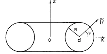
Figure 1.The poloidal current flowing on the surface of a torus.
Figure 2.The coordinatesR˜andψparametrizing the torus.
3.3. Electromagnetic field of the toroidal solenoid
Consider the poloidal current flowing on the surface of a torus (figure 1)
jT = −gc
4πnψ
δ(R− ˜R)
d+R˜cosψ nψ = nzcosψ− nρsinψ. (3.19) The coordinates R˜, ψ and φ are related to the Cartesian coordinates as follows:
x=(d+R˜cosψ)cosφ y=(d+R˜cosψ)sinφ
z= ˜Rsinψ. (3.20) The conditionR˜=Rdefines the surface of a particular torus (figure 2). ForR˜ fixed andψ, φvarying, the pointsx , y, z given by (3.20) fill the surface of the torus(ρ−d)2+z2=R2.
The choice ofj0in the form of (3.19) is convenient, because in
the static case a magnetic fieldHequalsg/ρinside the torus and vanishes outside it. In this case,gmay also be expressed through either the magnetic fluxpenetrating the torus or the total numberNof turns in a toroidal winding and the current
Iin a particular turn:
g=
2π(d−√d2−R2) =
2NI
c .
Let the current in a TS winding periodically change with time:
j= j0exp(iωt). Since
r× jT = 4gcπδ(R˜−R)nφ
and
rjT = gcd4sinπ ψ δ(
˜
R−R) d+Rcosψ one has
div(r× j)=0 alm(M)=0 alm(E)=0.
Therefore,
A= −4πik
c
Al(E)al(E)
H = −4πk2
c
Al(M)al(E)
E= −4πk2
c
Al(E)al(E) (3.21)
(Ais the vector potential). From the facts that: (i)rH = 0 and (ii)PAl(M)= (−1)lAl(M), it follows [15, 17] that the radiation field of a TS is of electric type.
The electric form factoral(E)for the radiating TS is equal to
al(E)=1
4gcdRk
2l+ 1
πl(l+ 1)Il
Il=
2π
0
jl(ky)Pl(x)sinψdψ (3.22) wherey = [d2 +R2+ 2dRcosψ]1/2 andx = Rsinψ/y.
It easy to check thatal(E)=0 forleven. Let the current time dependence be cosωt. Then the EMF is given by the real parts ofA,EandH:
Aθ = gdRk
2
2
1
l(l+ 1)IlP
1
l{[(l+ 1)jl−1−ljl+1]
×sinωt−[(l+ 1)nl−1−lnl+1] cosωt}
Ar= gdRk2r
(2l+ 1)IlPl(jlsinωt−nlcosωt)
Hφ=gdRk
3
2
2l+ 1
l(l+ 1)IlP
1
l(nlcosωt−jlsinωt)
Eθ = −gdRk
3
2
1
l(l+ 1)IlP
1
l{[(l+ 1)jl−1−ljl+1]
×cosωt+ [(l+ 1)nl−1−lnl+1] sinωt}
Er= −gdRk
2
2r
(2l+ 1)IlPl(jlcosωt+nlsinωt). (3.23) The number ofal(E)contributing to the sums in (3.23) is the same as for current loop: it should be slightly greater than 0.7kd.
Consider the following particular cases. (1) In the static limit (k→0) one obtains
Il→ k l
(2l+ 1)!!Cl al(E)→
gcdRkl+1
4(2l+ 1)!!
2l+ 1
πl(l+ 1)Cl
Tlm=δm0Tl Tl=
gdR√l
2(l+ 1)Cl
Cl=
2π 0
ylP l
Rsinψ
y
sinψdψ (3.24) whereTlmis the same as in (3.5). This integral can be taken in a closed form. We give its value only forl=1
C1=πR a1(E)=
πgdR2k2c
4√6π . The EMF strengths of the TS decrease ask2
Hφ∼ −gdRk2
1
l(l+ 1) 1
rl+1ClP 1
Eθ ∼ −gdRk
2
2 ct
Cl
l+ 1 1
rl+2P 1
l
Er∼ gdRk
2
2 ct
ClPlr1l+2. (3.25)
On the other hand, the vector potential of a TS does not vanish in the static limit
Aθ → −gdR2
Cl
l+ 1P
1
l
1
rl+2
Ar→gdR2
1
rl+2ClPl. (3.26)
The linear time dependence inE(forωt1) arises when one differentiates the cosωtterm inAand then letωgo to zero. For the infinitely thin TS (Rd),Clis reduced to
C2n+1=πRd2n(−1)n
(2n+ 1)!! 2nn! .
(2) Infinitely small toroidal solenoid (kd 1). Obviously, only thel=1 term contributes to sums in (3.23)
I1=
πkR
3 a1(E)=
πgdR2k2c
4√6π
Er =πgdR
2k2
2r2 cosθ
cosψ− 1
krsinψ
Eθ = πgdR
2k3
4r sinθ
sinψ
1− 1
k2r2
+ 1
krcosψ
Hφ= πgdR
2k3
4r sinθ
sinψ+ 1
krcosψ
. (3.27) For estimations, let the major radiusdof a TS be 10 cm. We rewrite the conditionkd1 in the wavelength language
2πd
λ ≈
60
λ 1.
This means that equations (3.27) will work forλ5m. (3) Infinitely thin toroidal solenoid (Rd). Taking into account the fact that
P2n+1(x)→ −P21n+1(0)x for x→0
one obtains
I2n+1= −R
dP
1
2n+1(0)D2n+1
D2n+1=
2π 0
j2n+1(ky)sin2ψdψ
a2n+1(E)= −
1 4gcR
2k
4n+ 3
π(2n+ 1)2(n+ 1)P
1
2n+1(0)D2n+1.
(3.28) ForRd(but for arbitrarykdandkR)D2n+1can be taken
in a closed form (see the appendix):
D2n+1
=π{J0(kR)j2n+1(kd)−12J2(kR)[j2n+3(kd)+j2n−1(kd)]}.
(3.29) If, in addition,kR1, then
D2n+1=πj2n+1(kd)
and
a2n+1(E)
= −π 4gcR
2k
4n+ 3
π(2n+ 1)2(n+ 1)P
1
2n+1(0)j2n+1(kd).
(3.30) On the other hand, ifkR1, then
D2n+1
= 2
kd
2π
kRcos kR− π
4
[(n+ 1)j2n+2(kd)+nj2n(kd)]
(3.31) (we cannot substitute instead of J2n(kd) and J2n+2(kd)
their asymptotic values, since the presence of J2n(kd) and
J2n+2(kd) guarantees the convergence of electromagnetic
strengths, (3.23)).
Forkd 1, equations (3.27) are not applicable. For example, ford=10 cm andλ=1cm,kd ≈60. The possible outcome is to take the minor radius of a TS as small as possible. Equations (3.23) withal(E)given by (3.28) and (3.29) are valid for arbitrary frequencies ifR 2 cm (ford =10 cm). The advantage of electric form factors (3.28) and (3.29) is that they do not involve integration, which is very cumbersome for high frequencies.
(4) Large distances (kr1). Then,
Eθ =Hφ= −gdRk
2
4r sinψ ×(−1)n 4n+ 3
(2n+ 1)(n+ 1)I2n+1P
1
2n+1 (3.32)
Er= gdRk2r2 cosψ
(4n+ 3)(−1)nI2n+1P2n+1.
The energy flux through the sphere of the radiusris
Sr = c
4πr
2
d1 EθHφ
=c
gdRk2sinψ
2
2
4n+ 3 2(n+ 1)(2n+ 1)I
2
2n+1. (3.33)
Correspondingly, the average energy lost for the period is
Sr= c
2
gdRk2
2
2
4n+ 3 2(n+ 1)(2n+ 1)I
2 2n+1.
3.3.1. Interaction of a TS with an external EMF. The interaction of a TS with external EMF is given by
U = −1
c
jTAextdV. (3.34)
Since divjT = 0, the poloidal current (3.19) flowing on the surface of the torus can be represented in the form [25]
jT =curlM divM =0
M= nφ4gcπρ3 R−
(ρ−d)2+z2 divM =0.
Figure 3.The poloidal currentjflowing on the surface of a torus is equivalent to the magnetizationM confined to the interior of the torus and to the toroidizationTdirected along the axis of the torus.
part of figure 3). Since divM =0, the magnetizationM, in its turn, can be written as
M=curlT divT=0 (3.36) where
T = nzT T = gc
4π
3 d−R2−z2−ρln d+
√
R2−z2
d−√R2−z2
+3 d+R2−z2−ρ3 ρ−d+R2−z2
×lnd+ √
R2−z2
ρ
. (3.37) Thus,T differs from zero in two space regions (see the lower part of figure 3) as follows.
(a) Inside the torus hole defined as 0ρd−√R2−z2,
whereT does not depend onρ
Tz= gc
4πln
d+√R2−z2
d−√R2−z2. (3.38)
(b) Inside the torus itself (d − √R2−z2 ρ d +
√
R2−z2) where
T = gc 4πln
d+√R2−z2
ρ . (3.39)
In other space regions,T =0. Therefore,
jT =curl curlT divT =0. (3.40)
Substituting (3.40) into (3.34), one obtains
U = −1
c2
˙
ETdV
(the dot aboveEdenotes time derivative). For distances large compared with the large radius of a TS
U = −1
c2 ˙ E
TdV. (3.41)
Despite the fact that T is rather complicated, the volume integral looks very simple
TdV = nzπcgdR
2
4 . (3.42) Physically, equations (3.35), (3.36) and (3.40) mean that the poloidal currentjgiven by (3.35) is equivalent (i.e. produces the same magnetic field) to the toroidal tube with magnetization
M defined by (3.36) and to toroidizationT given by (3.37). This is illustrated in figure 3. Obviously, these equations generalize Ampere’s hypothesis.
Now let the minor radiusRof a torus tend to zero (this corresponds to an infinitely thin torus). Then, the second term in (3.37) drops out, while the first one reduces to
T → gc
2πd3(d−ρ)
R2−z2. (3.43)
For infinitesimalR
R2−z2→1 2πR
2δ(z).
Therefore, in this limit,
j =curl curlT T = nzgcR
2
4d δ(z)3(d−ρ). (3.44) That is, the vectorT is confined to the equatorial plane of a torus and is perpendicular to it. Let nowd →0 (in addition toR→0). Then,
1
d3(d−ρ)→ d
2ρδ(ρ)
and the current of an elementary (i.e. infinitely small) TS is
j =curl curlT T = 14πcgdR2δ3(r)nz. (3.45) Let now the dependence of the current flowing in the toroidal solenoid befT(t), i.e.
JT =fT(t)curlnTδ3(r). (3.46) (the factor 1
4πcgdTR
2is included inf
T(t)). Then, the EMF
potentials and field strengths are given by
AT =c13r
−nTGT +r12r(rnT)FT
ET = c14r
nTG˙T −r12r(rnT)F˙T
HT = 1
4c3r(r× nT)D¨T (3.47)
where the functionsDT = D(fT),FT = F (fT)andGT =
G(fT)are defined by (3.18). WhenfTis independent oft, the
EMF strengths are zero, only the vector potential survives
AT = − 1
4cr3fT
nT −r32r(rnT)
.
3.3.2. Toroidal solenoids with a more realistic winding.
Usually, the toroidal coil twists along the torus surface having not only anψcomponent, but also anφcomponent parallel to the torus equatorial line. Then, the total density is given by
j =cosαjT + sinαjL (3.48) wherejLandjTare given by (3.6) and (3.19), respectively, and
αis the inclination angle of the currentjtowards the vector
nψ.
Since the EMF is a linear function of the current density, it is given by
E=cosαET + sinαEL H =cosαEH+ sinαHL (3.49) whereEL,HLandET,HT are the EMFs of the current loop and TS given by (3.9) and (3.23), respectively. Forα = 0 andα = π/2 the EMF (3.49) is transformed either into an EMF (3.23) of a TS or an EMF (3.9) of a current loop.
However, if there is a need to create pure toroidal EMF (3.23), then one should somehow compensate thenφ component ofj. For this, after finishing the toroidal winding (3.48) (i.e. when the last turn of the toroidal winding meets the first one), one closed turn lying in the equatorial torus plane and having the direction opposite tonφshould be added. Another possibility is to use a winding consisting of an even number of layers. If the directions of coils in the even and odd layers differ by the sign ofα, thenjφ current components of even and layers compensate each other and only thejψcomponent survives.
3.4. Historical remarks on TSs
TSs play an important role in physics and technology. As the simplest three-dimensional topologically non-trivial objects, they have been used for the experimental verification of the Aharonov–Bohm effect [26]. The corresponding calculations were performed in [27]. They possess a number of non-trivial characteristics such as toroidal [18, 28] and ‘hidden’ [29] moments. Exact vector potentials of finite static TSs were evaluated by Luboshitz and Smorodinsky [30], in a non-standard gauge, and in [31], in a Coulomb gauge. Similarly to the static magnetic TSs outside which the EMF strengths disappear, but the magnetic vector potential differs from zero, there are electric TSs outside which the EMF strengths are zero but non-trivial electric vector potentials differ from zero [25, 32]. Furthermore, there exists the toroidal Aharonov–Casher effect which describes quantum (not classical) scattering of toroidal dipoles by the electric charge [33].
Turning to TSs with time-dependent currents, one should mention two papers by Page [34]. However, his EMF strengths were presented in the integral form, unsuitable for practical applications. The EMF of TSs for a number of time dependences were studied in [35]. Unfortunately, the most interesting case of a periodical current was considered for a very special case of an infinitely small TS. The multipole expansion of the EMF for a TS with periodical current was given in [19, 36]. However, these presentations were too schematic, without practical applications. Equations (3.47) for the EMF of an infinitely small TS was earlier been obtained
by Nevessky [37] and, also, in [38]. Their generalization for more complicated toroidal configurations is given in [39]. In the same reference, as well as in [25], the charge– current toroidal configurations were found outside which non-trivial (that is unremovable by a gauge transformation) time-dependent electromagnetic potentials were different from zero despite the vanishing EMF strengths. This makes possible the performance of experiments investigating the time-dependent Aharonov–Bohm effect. All these studies are summarized in [40].
What is new in this section? It seems that general equations (3.23) defining EMFs of TS and corresponding particular cases (3.24)–(3.33) were not considered previously. We briefly enumerate the applications of TSs as follows. (a) Toroidal transformers are very effective since the leakages
of the EMF into the surrounding space are very small. (b) TSs are widely used in modern accelerators. Being placed
along the circumference, they generate electromagnetic field concentrated inside the torus holes (see e.g. [25], where the exactly soluble configuration of a TS producing a time-dependent EMF confined to the interior of a circular tube was considered).
(c) According to [41] ‘Air-cored toroidal inductors are used in power electronic circuits because they are relatively easy to make, they do not saturate and they do not produce troublesome external magnetic fields.’
(d) Finally, one should mention Birkeland’s electromagnetic gun (see, e.g., [42]) in which the set of toroidal solenoids are used for the acceleration of an iron bullet. The modern version of Birkeland’s gun is realized in US Star Wars
programme, officially known as the Strategic Defence Initiative.
4. EMF of an electric dipole
Consider two point charges at the points±adn. Their charge density is given by
ρd =e[δ3(r−adn) −δ3(r+adn) ].
For an infinitely small dipole, this takes the form
ρd = −2ea(n∇)δ3(r) ∇i= ∂x∂ i.
Now let the charge density depend on time
ρd =f (t)(n∇)δ3(r)
(factor−2eais included inf (t)). The corresponding current density is given by
jd= −f (t)˙ nδ 3(r). (4.1)
The following EMF strengths correspond to these densities:
Hd= c21r2(r× n)D˙d
Ed= c12r
nGd−r12(nr)rF d
Now let the time dependence of the charge density be cosωt:
ρd = −2eadcosωt(n∇)δ3(r)
jd= −2eadωsinωtnδ 3(r). (4.3)
For the unit vectornalong thezaxis, one obtains
Hdφ = −2eadk
2
r sinθ
cosψ−sinψ
kr
Edθ = −2eadk
2
r sinθ
cosψ
1− 1
k2r2
−sinψ
kr
Er d=
4eadk
r2 cosθ
sinψ+ 1
krcosψ
ψ=kr−ωt.
(4.4) In the static limit (k→0) one obtains the field of an electric dipole
Edθ →2ard3esinθ Edr→4ear3dcosθ Hdφ →0. For the oscillating electric dipole with a finitead, oriented along thezaxis
ρd=i exp(iωt)ρd0
ρd0=
e
2πa2
dsinθ
δ(r−ad)[δ(θ)−δ(π−θ)]
jd= nrjd jd= −ωexp(iωt)jd0
jd0= e
2πr2sinθ3(ad−r)[δ(θ)−δ(π−θ)] (4.5)
If we desire to obtain, in the static limit, the static electric densi