Abstract—In ongoing investigation the unsteady magneto-hydrodynamics flow and heat transfer with viscous dissipation of a third grade fluid passed between two long parallel flat porous plates is discussed. With the physical assumptions a coupled system of non-linear partial differential equation is procured as governing MHD flow and heat transfer problem, which is then transformed to a system of non-linear algebraic equations by descretising using fully implicit finite difference scheme and solved numerically by damped-Newton method. Finally the problem is coded using MATLAB programming. The numerical results which characterize the imposing physical parameters are described through various graphs. The foremost finding of the present study is that out two elastic parameters the visco-elastic parameter𝜶 has a dominant role over the non-Newtonian parameter and has a control over reducing thevelocity flow of third grade fluid. Again more viscous dissipation energy is generated when the parameter values of E increases, as a result temperature profile increases.
Index Terms— magneto-hydrodynamics, unsteady flow, viscous-dissipation, third grade fluid, Porousplates.
I. INTRODUCTION
HEstudy of non-Newtonian fluids is intensified due to its numerous application in industry and engineering. To describe various characteristics of non-Newtonian fluid different constitutive fluid models are developed. Second grade fluid model is one of the simplest subclass of these models which is capable of describing normal stress differences. But this model is inadequate to describe shear thinning/thickening phenomenon observed in many non-Newtonian fluids as described by Joseph and Fosdick(1973), Beavers and Joseph(1975). Such characteristics of visco-elastic fluids can be predicted by third grade fluid model. Many researcher like Ariel(2002), Hayat et al.(2002), Hayat et al.(2008), Abbasbandy et al.(2008), Sahoo(2009), Narain and Kara(2010),Sahoo and Poncet(2011), Nayak et al.(2012), Gital et al.(2014), Awais(2015),O Samuel and D Oluwole(2015),O Samuel and Falade(2015), Nayak et al.(2016), Qian and Cai(2018), are involved in studying the non-Newtonian fluid models due to its important technological application.
Recently Wang et al.(2016) have studied flow and heat transfer of third grade fluid within two micro parallel plates in presence of magnetic field and an externally imposed electrical field. The problem is analyzed both by analytic
Manuscript received June 01, 2018; revised March 26, 2019.
I. Nayak is with the Veer Surendra Sai University of Technology (VSSUT), India (phone: +91-9937357213; e-mail: [email protected]).
and numerical method. Then finally a comparison is done between these solutions. Okoya(2016) have analyzed the criticality and transition of a third grade fluid through a pipe with Reynolds number viscosity. The steady incompressible flow of an exothermic reactive third grade fluid is solved numerically and discussed for both cases of viscosity and Reynolds number viscosity model. Carapau and Corria (2017) have discussed the numerical simulation of third grade fluid in a tube through a contraction. They used numerical simulation to analyze unsteady flow over a finite set or a tube with contraction is performed. Opangue et al.(2017) have investigated entropy generation of hydro-magnetic couple stressfluid flow through a channel filled with a non—Darcian medium. Then they solve the coupled fourth order non-linear set of differential equation using Adomain decomposition method and differential transform method. Carapau et al.(2017) used a non-dimensional hierarchical approach to solve generalized third grade fluid with shear dependent visco-elastic effect model. They consider the particular case of a flow through a straight and rigid tube with constant circular cross section. Then a real three dimensional flow problem is reduced to exact three dimensionalsystems as an ordinary differential equation and final solution is obtained using the Runge-Kutta method.
In present study, it is attempted to analyze the most generalized case of unsteady magneto-hydrodynamics flow and heat transfer of a third grade fluid passingwithin an infinite porous channel with viscous dissipation. Where the upper plate is fixed and lower plate suddenly gets in motion with a velocity whichvaries with respect to time. A comparison study is made by taking smaller as well as larger values of all emerging physical parameters. Now a day, study of non-Newtonian fluid with magnetic field is used in different branches of technology as exploiting liquid metal, bio-medical engineering, magneto-hydrodynamic power generation and many more. Thus this study is advantageous because of its important technological application and efficacious mathematical features. Also to my knowledge so far in above cited studies the present numerical investigation is not done.
A fully implicit finite difference scheme is used to convert governing coupled non-linear partial differential equation into a system of non-linear algebraic equations and then numerical solution is obtained using quadratic convergent damped Newton method. The advantage of the employed scheme is that, it is valid for small as well as large value of elastic parameters. Further this method does not require repeated derivation of the problem for every change
Numerical Study of MHD Flow and Heat
Transfer of an Unsteady Third Grade Fluid with
Viscous Dissipation
Itishree Nayak
T
IAENG International Journal of Applied Mathematics, 49:2, IJAM_49_2_14
in boundary condition.
Rest of the paper is organized successfully. Section 2 is concerned with theproblem formulation. The convergence and stability of the scheme for the MHD flow and heat transfer is discussed in section 3. Section 4 gives a detailed account regarding impact of several physical parameters on fluid flow with graphical representation. Section 5 concludes the paper.
II. CONSTRUCTION OF PROBLEM
The stress tensor P for an incompressible homogeneous and thermodynamically compatible third grade fluid by Fosdick and Rajagopal (1980) is
𝑃 = −𝑝𝐼 + 𝜇𝐴1+ 𝛼1𝐴2+ 𝛼2𝐴12+ 𝛽3(𝑡𝑟𝐴12)𝐴1 (2.1) 𝑤𝑒𝑟𝑒 𝜇 = 𝑣𝑖𝑠𝑐𝑜𝑠𝑖𝑡𝑦
𝛼1, 𝛼2= 𝑛𝑜𝑟𝑚𝑎𝑙 𝑠𝑡𝑟𝑒𝑠𝑠 𝑚𝑜𝑑𝑢𝑙𝑖 𝛽3= 𝑖𝑔𝑒𝑟 𝑜𝑟𝑑𝑒𝑟 𝑣𝑖𝑠𝑐𝑜𝑠𝑖𝑡𝑦 𝑝 = 𝑝𝑟𝑒𝑠𝑠𝑢𝑟𝑒
𝐼 = 𝑖𝑑𝑒𝑛𝑡𝑖𝑡𝑦𝑡𝑒𝑛𝑠𝑜𝑟
𝐴1, 𝐴2= 𝑘𝑖𝑛𝑒𝑚𝑎𝑡𝑖𝑐𝑎𝑙𝑡𝑒𝑛𝑠𝑜𝑟, defined by Rivlin and Erickson (1995)
Here lower plate is taken along x'-axis and y'-axis is normal to it. The upper plate isspecified by y'=1. Let both plates can extends to infinite in either sides of the x'-axis, where the upper plate is assumed to be fixed and lower plate moves witha time varying velocity F(t). Let V > 0 indicate the suction velocity at the plate. A transverse uniform magnetic field with strength 𝐵0is applied at the lower plate.
With the above physical assumptions and the stress components given in eq.(2.1) the governing third grade flow equation becomes
𝜌 𝜕𝑤𝜕𝑡′′+ 𝑉
𝜕𝑤′
𝜕𝑦′ = 𝜇
𝜕2𝑤′
𝜕𝑦′2 + 𝛼1 𝜕3𝑤′
𝜕𝑦′2𝜕𝑡′+ 6𝛽3( 𝜕𝑤′ 𝜕𝑦′)
2 𝜕2𝑤′ 𝜕𝑦′2+ 𝛼1𝑉𝜕
3𝑤′
𝜕𝑦′3− 𝜎𝐵0 2
𝜌 𝑤′ (2.2) With subjected initial and boundary conditions are
𝑡′= 0: 𝑤′= 0, ∀𝑦′
𝑡′> 0: 𝑤′= 𝐹(𝑡) 𝑓𝑜𝑟𝑦 = 0 (2.3) 𝑤′= 0 𝑓𝑜𝑟𝑦′= 1
Where 𝐹 𝑡 = 𝐴sin(𝑤′𝑡′) 𝑦 = 𝜗𝑇𝑦′ , 𝑡 =𝑡𝑇′, 𝑤 =𝑤𝐴′ , 𝜃 = 𝜃
′−𝜃
1
𝜃2−𝜃1 , 𝜔 = 𝜔′𝑇(2.4)
𝑅𝑒 =𝑉 𝑇 𝜗 , 𝛼 = 𝛼1 𝜗𝑇𝜌 , 𝛾 =
6𝛽3𝐴2
𝜌𝜗2𝑇 ,𝑚2=
𝜎𝐵02𝑇 𝜌 , 𝑝𝑟 =𝜗𝜌 𝑐𝑘𝑝 , 𝐸 = 𝐴
2
𝑐𝑝(𝜃2−𝜃1)
.
Where Re – local Reynolds number, - visco-elastic parameter, - third grade elastic parameter, m- Hartmann number, Pr – Prandtl number, E –viscous dissipation parameter, 𝜗 – kinematic coefficient of viscosity. A= constant.
Then the non-dimensionalized field equation of velocity can be obtained as
𝜕𝑤 𝜕𝑡
+ 𝑅𝑒
𝜕𝑤 𝜕𝑦
=
𝜕2𝑤 𝜕𝑦2
+ 𝛼
𝜕3𝑤 𝜕𝑦2𝜕𝑡
+ 𝛾(
𝜕𝑤 𝜕𝑦
)
2 𝜕2𝑤
𝜕𝑦2
+
𝑅𝑒𝛼
𝜕𝜕𝑦3𝑤3− 𝑚
2𝑤
(2.5)Along with the initial and boundary condition as follows: 𝑡 = 0 ∶ 𝑤 = 0 , ∀𝑦
𝑡 > 0 ∶ 𝑤 = sin 𝜔𝑡 , 𝑓𝑜𝑟𝑦 = 0 (2.6)𝑤 = 0, 𝑓𝑜𝑟𝑦 = 1 The thermal field equation for the thermodynamically compatible third grade fluid with viscous dissipation 𝜌𝑐𝑝 𝜕𝜃
′
𝜕𝑡′+ 𝑉
𝜕𝜃′
𝜕𝑦′ = 𝑘
𝜕2𝜃′
𝜕𝑦′2+ 𝜇
𝜕𝑤′
𝜕𝑦′
2
+ 𝛼1 𝜕
2𝑤′
𝜕𝑦′𝜕𝑡′
𝜕𝑤′
𝜕𝑦′ +
𝛼1𝑉 𝜕
2𝑤′
𝜕𝑦′2
𝜕𝑤′ 𝜕𝑦′ + 2𝛽3
𝜕𝑤′ 𝜕𝑦′
4
+ 𝜎𝐵02𝑤′ (2.7) With the initial and boundary condition which are subjected to the equation (2.7) are
𝑡′= 0 ∶ 𝜃′= 0 ∀𝑦′ 𝑡′> 0 ∶ 𝜃′= 𝜃
2𝑓𝑜𝑟𝑦′= 0 (2.8) 𝜃′ = 0𝑓𝑜𝑟𝑦′= 1
ρ = densityoffluid, σ = electrical conductivity, μ = viscosity, cp= specificheat, k =
thermalconductivity andθ′= temperature .
Non-dimensionalized field equation of energy with initial and boundary condition is secure as
𝜕𝜃 𝜕𝑡 + 𝑅𝑒
𝜕𝜃 𝜕𝑦 =
1 𝑝𝑟
𝜕2𝜃 𝜕𝑦2+ 𝐸
𝜕𝑤 𝜕𝑦
2
+ 𝛼𝐸 𝜕 2𝑤
𝜕𝑦𝜕𝑡 𝜕𝑤
𝜕𝑦
+𝛼𝑅𝑒𝐸 𝜕𝜕𝑦2𝑤2 𝜕𝑤𝜕𝑢 +𝛾𝐸3 𝜕𝑤𝜕𝑦 4 +𝐸𝑚2𝑤 (2.9)
With the initial and boundary conditions: 𝑡 = 0 ∶ 𝜃 = 0, 𝑓𝑜𝑟𝑎𝑙𝑙𝑦
𝑡 > 0 ∶ 𝜃 = 1, 𝑓𝑜𝑟𝑦 = 0 (2.10) 𝜃 = 0, 𝑓𝑜𝑟𝑦 = 1
[image:2.595.64.276.452.547.2]The above system of non-linear coupled differential equations is solved under the relevant initial and boundary conditions with the help of implicit finite difference scheme. Then the numerical solution of the system is obtained using above said method described in Conte, De Boor (1980).
Fig. 0, Fluid flow between porous plates
Y=0
Y=1
B
0Porous Plate
Porous Plate
Third grade Fluid
IAENG International Journal of Applied Mathematics, 49:2, IJAM_49_2_14
III. NUMERICAL SOLUTION METHOD
The equation (2.5), (2.6), (2.9) and (2.10) are solved by finite difference scheme of crank- Nicolson type. Taking a uniform mesh of step h and time step ∆t the grid points generated are
𝑦𝑗 , 𝑡𝑗 = 𝑖 , 𝑗∆𝑡 , 𝑖 = 0,1,2, … , 𝑁 + 1, 𝑗 = 0,1,2, … , 𝑀 − 1
Following notations and difference approximations to the derivative are taken at different nodes asfij’s.
Notations: 𝑓1𝑖𝑗 = 𝑤𝑖+1𝑗 − 𝑤𝑖−1𝑗
𝑓2𝑖𝑗 = 𝑤𝑖+1𝑗 − 2𝑤𝑖𝑗+ 𝑤𝑖−1𝑗
𝑓3𝑖𝑗 = −𝑤𝑖−2𝑗 + 2𝑤𝑖−1𝑗 − 2𝑤𝑖+1𝑗 + 𝑤𝑖+2𝑗
𝑓3𝑖′𝑗 = −3𝑤𝑖−1𝑗 + 10𝑤𝑖𝑗− 12𝑤𝑖+1𝑗 + 6𝑤𝑖+2𝑗 − 𝑤𝑖+3𝑗
𝑓3𝑖′′𝑗 = 𝑤
𝑖−3𝑗 − 6𝑤𝑖−2𝑗 + 12𝑤𝑖−1𝑗 − 10𝑤𝑖𝑗+ 3𝑤𝑖+1𝑗
The difference approximation to the derivatives at nodes ih , j∆t , i = 1,2, … , N + 1 and
𝑗 = 0,1, … , 𝑀 + 1arewritten as
𝜕𝑤
𝜕𝑡
≈
𝑤
𝑖𝑗 +1− 𝑤
𝑖𝑗∆𝑡
𝜕𝑤𝜕𝑦
≈
𝑓1𝑖𝑗 +1+𝑓1𝑖𝑗 4
𝜕2𝑤 𝜕𝑦2
≈
𝑓2𝑖𝑗 +1+𝑓2𝑖𝑗
22
(3.1)
𝜕3𝑤𝜕𝑦3 ≈
𝑓3𝑖𝑗 +1+ 𝑓3𝑖𝑗 23
𝜕
3𝑤
𝜕𝑦
2𝜕𝑡
≈
𝑓
2𝑖𝑗 +1− 𝑓
2𝑖𝑗
2∆𝑡
At the point (1, j∆𝑡) and (N, 𝑗∆𝑡 ) the third grade derivative 𝜕3𝑤
𝜕𝑦3 is replaced respectively by
𝑓3𝑖′𝑗 +1+𝑓3𝑖′𝑗 23 and
𝑓3𝑖′′𝑗 +1+𝑓3𝑖′′𝑗 23 .
Here the difference scheme is seen to be unconditionally stable and has second order convergence in time and space. With the implementation of above said notations in (3.1), the governing equation of velocity is discretized as
𝑤𝑖𝑗 +1−𝑤𝑖𝑗 ∆𝑡 + 𝑅𝑒
𝑓1𝑖𝑗 +1+𝑓1𝑖𝑗
4 =
𝑓2𝑖𝑗 +1+𝑓2𝑖𝑗 22 + 𝛼
𝑓2𝑖𝑗 +1−𝑓2𝑖𝑗 2∆𝑡 +
𝑅𝑒𝛼𝑓3𝑖𝑗 +1+𝑓3𝑖𝑗
23 +
𝛾
324(𝑓1𝑖𝑗 +1+ 𝑓1𝑖𝑗)2(𝑓2𝑖𝑗 +1+ 𝑓2𝑖𝑗)−𝑚2( 𝑤𝑖𝑗 +1+𝑤𝑖𝑗
2 )
(3.2) For i = 2,3,...,N-1, j=0,1,2,...,M.
The initial and boundary conditions in discretized form as follows:
𝑤𝑖0= 0, 𝑖 = 0,1, … , 𝑁 + 1
𝑤0𝑗 = sin 𝜔𝑗∆𝑡and (3.3) 𝑤𝑁+1𝑗 = 0, 𝑗 = 1, … , 𝑀
The governing equation of energy in discretized form is written as
𝜃𝑖𝑗 +1−𝜃𝑖𝑗
∆𝑡 +
𝑅𝑒 4 𝜃𝑖+1
𝑗 +1− 𝜃
𝑖−1𝑗 +1 + (𝜃𝑖+1𝑗 − 𝜃𝑖−1𝑗 ) = 1
𝑝𝑟22 𝜃𝑖+1
𝑗 +1− 2𝜃
𝑖𝑗 +1+ 𝜃𝑖−1𝑗 +1 + 𝜃𝑖+1𝑗 − 2𝜃𝑖𝑗+ 𝜃𝑖−1𝑗 +
𝐸(𝑓1𝑖𝑗 +1+𝑓1𝑖𝑗
4h )
2+ 𝛾𝐸
3×162×4(𝑓1𝑖𝑗 +1+ 𝑓1𝑖𝑗)4+ 𝐸𝛼
82∆𝑡 𝑓1𝑖𝑗 +1+ 𝑓1𝑖𝑗 𝑓1𝑖𝑗 +1− 𝑓1𝑖𝑗 +𝛼𝑅𝑒𝐸83 𝑓1𝑖𝑗 +1+ 𝑓1𝑖𝑗 𝑓2𝑖𝑗 +1+ 𝑓2𝑖𝑗 +
𝐸𝑚2(𝑤𝑖𝑗 +1+𝑤𝑖𝑗
2 )
(3.4)
With initial and boundary conditions on θ in discretised form
𝜃𝑖0= 0, 𝑖 = 0,1,2, … , 𝑁 + 1
𝜃0𝑗 = 1 𝑎𝑛𝑑 (3.5) 𝜃𝑁+1𝑗 = 0, 𝑗 = 1,2, … , 𝑀.
To impose the boundary conditions at infinity, we choose N so that the absolute difference of two solutions obtained by assuming the boundary conditions at∞ to hold at 𝑁 + 1 , 𝑗∆𝑡 𝑎𝑛𝑑 ( 𝑁 + 2 , 𝑗∆𝑡) successively, so that the difference between the two consecutive solutions obtained is less than a prescribed error tolerance∈ given in Jain (1984). A tri-diagonal system of equations is obtained after rearrangement of energy equation. Then it is solved using special form of Gaussian elimination method with the help of initial velocities which are obtained again by solving the tri-diagonal system for velocity formed by making the parameter m, αandγbecome zero in constitutive equation of velocity given in eq.(3.2). Similarly initial choice of temperature is made converting the energy equation into a tri-diagonal system by making the parameter Eand α become zero in eq.(3.4) and then it is solved using the exponentially fitted scheme described in Morton(1996).
Then the system of non-linear equations for velocity (3.2) with its initial and boundary conditions (3.3) is solved by damped-Newton method. For implementation of this method the residuals (Ri, i = 0,1,2, … , N) and the non-zero elements of the Jacobian matrix ∂Ri
∂wj , i = 1,2, … , Nandj = 1,2, … , M of the system are computed. The above method isquadratically convergent and a new approximation 𝑥𝑚+1being accepted as xm
+ h 2 i for some suitable i, only when it satisfies 𝑓 𝑥𝑚+ 2 𝑖
2< 𝑓 𝑥𝑚
2 ,otherwise the failure occur. This ensuresthere must be decrease in residual error after every iteration. Hence it establishes the convergence of the iteration scheme. The MATLAB coding for the above numerical scheme is verified with the existing result given in Conte, De Boor (1980) and the results are found to be correct up to 10−5. Hence the aforementioned iteration scheme is stable and convergent. Finally procure results are presented through
IAENG International Journal of Applied Mathematics, 49:2, IJAM_49_2_14
graphs and its physical concepts are described in following section.
IV. RESULTS&DISCUSSION
[image:4.595.76.267.182.335.2]The current investigation shows the unsteady MHD flow and heat transfer characteristics of third grade fluid placed between two porous plates subjected to a uniform magnetic field. Results are plotted graphically in fig-1 to fig-24 for different physical parameters.
[image:4.595.333.518.242.394.2]Fig. 1, Effect of on Velocity field ( = 3,Re=7, w=1, pr=.3, E=.7, m=7, n=100)
[image:4.595.78.262.374.522.2]Fig. 2, Effect of on Temp. field ( = 3,Re=7, w=1, pr=.3, E=.7, m=7, n=100)
Fig. 3, Effect of on Velocity field ( = 5,Re=10, w=1, pr=.3, E=.7, m=5, n=100)
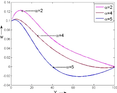
Fig-1, 2, 3, 4 (𝛼 > 1) it is observed that with increasing the second grade elastic parameter 𝛼values, elasticity of the fluid increases that reduces fluid velocity profile. A sudden
hike of velocity revealed near the upper plate and then velocity decreases towards the lower plate. Whereas a significant increase of temperature profile is observed throughout the flow field and the maximum effect is seen at the center of the plates.
Fig-5, 6(𝛼 < 1) illustrates a similar impact as to previous case for both the fields, which is obtained with the reduction of non-Newton parametric value γ to1 and magnetic parameter value m to 5 than the previous case.
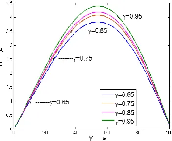
Fig-7, 8 (γ>1) Forlarge values of third grade elastic parameter γ, it is observed that velocity profile increases and temperature profile decreases with increase of the non-Newtonian parameter γ.
[image:4.595.331.518.431.581.2]Fig. 4,Effect of on Temp.field ( = 5,Re=10, w=1, pr=.3, E=.7, m=5, n=100)
Fig. 5, Effect of 𝛼on Velocity field ( = 1,Re=7, w=1, pr=.3, E=.7, m=5, n=100)
IAENG International Journal of Applied Mathematics, 49:2, IJAM_49_2_14
[image:4.595.71.261.567.718.2] [image:4.595.339.515.620.762.2]Fig. 6, Effect of 𝛼 on Temp. field ( = 1,Re=7, w=1, pr=.3, E=.7, m=5, n=100)
[image:5.595.337.513.242.386.2]Fig. 7, Effect of on Velocity field (𝛼 = 3, Re=8, w=1, pr=.3, E=.7, m=7, n=100)
[image:5.595.81.257.274.418.2]Fig. 8, Effect of on Temp (𝛼 = 3 ,Re=8, w=1, pr=.3, E=.7, m=7, n=100)
Fig. 9, Effect of on Velocity ( = 4, Re=8, w = 1, pr =.3, E =.7, m= 7, n = 100)
Fig. 10,Effect ofon Temp. ( = 4, Re = 8, w = 1, pr =.3, E =.7, m= 7, n = 100)
.
Fig. 11, Effect of on Velocity field ( = 3, Re = 8, w = 1, pr =.3, E =.7, m= 7, n = 100)
[image:5.595.339.514.421.559.2]Fig. 12,Effect of on Temp. ( = 3, Re = 8, w = 1, pr =.3, E =.7, m= 7, n = 100
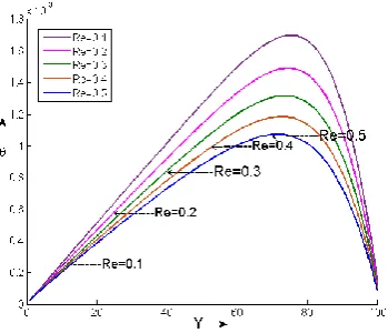
[image:5.595.78.259.444.584.2]Fig. 13, Effect of Re on Vel. ( = 3, = 3, w = 1, pr =.3, E=.7,m=5, n = 100)
Fig. 14, Effect of Re on Temp. ( = 3, = 3, w = 1, pr =.3, E =.7, m=5, n = 100)
IAENG International Journal of Applied Mathematics, 49:2, IJAM_49_2_14
[image:5.595.336.514.603.749.2] [image:5.595.80.258.621.763.2]Fig. 15, Effect of Re on velocity field ( = .01, = 1, w = 1, pr =.3, E =.7,m=0.5, n = 100)
Fig-9, 10 But when second grade elastic parameter value of 𝛼 raised to 4 keeping rest parameters fixed, a decreasing behavior of velocity profile is observed with increasing the values ofγ. Also it slow down the velocity as well as temperature profile and conforms that influence of second grade elastic parameter is more on velocity profile than third grade elastic parameter γ.
Fig-11, 12 (<1) Again for small values of third grade elastic parameter the momentum boundary layer thickness gradually decreases with increase of values. This might occur, because when values are small, the influence of second grade elastic parameter is more on flow field and that causes gradual deceleration of velocity profile. The effect is not pronounced near the boundary, but a noticeable effect is seen away from boundary. The temperature field increases with increase of the parameter values.
Fig. 16,Effect of Re on Temp. ( = .01, = 1, w = 1, pr =.3, E =.7,m=.5, n = 100)
Fig-13, 14(Re >1) Depict the impact of Reynolds number Re
on velocity and temperature field. It shows when values of
Re increases, viscous force of the fluid gradually increases
which causes decrease in both velocity as well as temperature profile at all points of the domain of fluid flow. Fig-15, 16(Re <1) Similar effect is seen on velocity and
temperature profile when Reynolds number values are less than 1 obtained along with a reduction inthe values of elastic parameters , and magnetic parameter m. Here the momentum and thermal boundary layer influence near the plates observed to be insignificant.
Fig. 17, Effect of m on velocity field ( = 3, = 3, Re = 7, w = 1, pr =.3,E=.7,n = 100)
[image:6.595.337.514.328.472.2]Fig-17, 18(𝑚 > 1) Show that velocity gradually decreases when magnetic parameter m values increases. Due to increase in magnetic field strength the transverse Lorentz force increases on flow field, which in turns reduces the fluid velocity. But a substantial increase is seen on temperature field
Fig.18, Effect of m on Temp. ( = 3, = 3, Re = 7, w = 1, pr =.3,E=.7, n = 100)
Fig. 19, Effect of m on vel. ( = 3, = 3, Re = 7, w = 1,pr=.3, E =.7, n = 100)
Fig-19, 20 (m< 1) Portray the effect of smaller magnitude magnetic field effect on velocity and temperature profile. It is observed here that the effect of Lorentz force become negligible and that provides less amount of resistance to the fluid flow, so a profound increase of velocity profile is seen. But the temperature field observed to be decreasing.
IAENG International Journal of Applied Mathematics, 49:2, IJAM_49_2_14
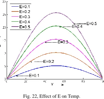
[image:6.595.82.257.453.603.2] [image:6.595.333.512.514.661.2]Fig-21, 22 recite the effect of viscous dissipation parameter
E on temperature profile. It is seen that temperature profile increases with increase of every value of viscous dissipation parameter E.
[image:7.595.85.260.145.287.2]So when E increases viscous dissipation heat generated is more which causes rise in the temperature field.
[image:7.595.341.513.154.318.2]Fig. 20,Effect of m on Temp. ( = 3, = 3, Re = 7, w = 1,pr=.3, E =.7, n = 100)
Fig. 21,Effect of E on Temp. ( = 2, = 3, Re = 7, w = 1, pr =.3,m = 7, n = 100)
Finally fig-23, 24 Depicts when 𝑝𝑟< 1 temperature profile decreases with increase of Prandtl number. Where the effect is noticeable near the boundary and gradually diminishes away from the boundary. For 𝑝𝑟 > 1 it is observed that when the parameter values increases, the temperature field decreases near the surface of the plate and then gradually increases away from the plate and that causes a cross over temperature profile.
V. CONCLUSION
This study analyses unsteady magneto-hydrodynamic flow and heat transfer of third grade fluid in a porous channel. The results are pictorially presented through several graphs and a comparison study is made between small and large values of physical parameters on velocity and temperature field. The imperative finding of the present study are as follows
Velocity profile decreases and temperature profile increases with increase of low as well as high values of second grade elastic parameter .
Velocity profile increases and temperature decreases with increase of low as well as high value of third grade elastic parameter when = 3.But the effect become opposite on both the fields
for valuesof become 4 or more and strengthening second grade elastic parameter to 4.
[image:7.595.90.244.320.463.2] Velocity decreases and temperature increases with increase of the magnetic parameter m values but on reduction of parametric values of m, a reversed effect is seen on both the fields.
Fig. 22, Effect of E on Temp.
( = 2, = 3, Re = 7, w = 1, pr =.3,m = 7, n = 100)
Fig. 23,Effect of Pr on Temp. ( = 3, = 3, Re = 9, w = 1, E =.7, m= 7, n = 100)
Fig. 24Effect of Pr on Temp. ( = 3, = 3, Re = 9, w = 1, E =.7, m= 7, n = 100)
Moreover when viscous dissipation factor E increases, temperature profile increases whatever the Eckert number E is large or small.
IAENG International Journal of Applied Mathematics, 49:2, IJAM_49_2_14
[image:7.595.339.512.337.493.2] [image:7.595.316.491.542.684.2]This means large values of visco-elastic parameter and magnetic parameter m create hindrance on fluid flow and slow down the velocity profile but the temperature field increases substantially.
REFERENCES
[1] S. Abbasbandy, T. Hayat, R. Ellahi, S. Asghar, ―Numerical results of a flow in third grade fluid between two porous walls,‖ Zeitschrift für
Naturforschung A, vol. 64, no. 1-2, pp.51-59, 2008.
[2] P. D. Ariel, ―Flow of third grade fluid through a porous flat channel,‖
Int. J. of Engg. Sci. vol. 41, no. 11, pp.1267-1285, 2002.
[3] M. Awais, ―Application of numerical inversion of the Laplace transform to unsteady problems of third grade fluid,‖ Applied
mathematics and computation, vol. 250, no. 1, pp.228-234, 2015.
[4] G. S. Beavers, D.D. Joseph, ―The rotating rod viscometer,‖ J. Fluid mech., vol. 69, no. 3, pp. 475-511, 1975.
[5] S. D. Conte, De Boor, C., Elementary numerical analysis an
algorithmic approach, McGraw-Hill, Inc, New-york, 1980,
pp.219-221.
[6] F. Carapau, P. Corria, ―Numerical simulations of third grade fluid on a tube through a contraction,‖ European journal of mechanics B/ fluids, vol. 65, no. 1, pp.45-53, 2017.
[7] F. Carapau, P. Corria., M. G. Luis, R. Conceicao, ―Axisymmetric motion of a proposed generalized non-Newtonian fluid model with shear-dependent visco-elastic effects,‖ IAENG Int. J. of applied
Mathematics, vol. 47, no. 4, pp. 361-370, 2017.
[8] R. L. Fosdick, K.R. Rajagopal, ―Thermodynamics and stability of fluids of third grade,‖ in Proc. of Royal society London-A, U.K., 369(1980), pp. 351-377.
[9] A. Y. Gital, M. Abdulhameed, C. Haruna, M. S. Adamu, B. M. Abdulhamid, A. S. Aliyu, ―Coutte flow of third grade fluid between parallel porous plates,‖ American journal of computational and
applied mathematics, vol. 4, no. 2, pp.33-44, 2014.
[10] T. Hayat, S. Nadeem, A.M. Siddiqui, ―Fluctuating flow of a third order fluid on a porous plate in a rotating medium,‖ Int.J. of
non-linear Mech., vol. 36, no. 6, pp.901-916, 2002.
[11] T. Hayat, N. Ahmed, , and M. Sajid, ―Analytic solution for MHD flow of a third grade fluid in a porous channel,‖ J. of comp. and app.
Maths., vol. 214, no. 2, pp.572-582, 2008.
[12] M. K. Jain, Numerical solution of differential equations, 2ED, Wiley Eastern, New Delhi, pp. 193-194.
[13] D. D. Joseph, R. L. Fosdick, ―The free surface on a liquid between cylinders rotating at different speeds,‖ Arch. Rat. Mech., Anal., vol. 49, no. 5, pp.321-401, 1973.
[14] K.W. Morten, Numerical solution of convection diffusion problems, Chapman and Hall, London, pp. 84-86.
[15] R. Narain, A. H. Kara, ―An analysis of the conservation laws for certain third grade fluids,‖ Nonlinear analysis: Real world applications, vol. 11, no. 4, pp. 3236-3241, 2010.
[16] I. Nayak, A. K. Nayak, S. Padhy, ―Numerical solution for the flow and heat transfer of a third grade fluid past a porous vertical plate,‖
Adv. St. in the The. Phy. , vol. 6, no. 13, pp.615-624, 2012.
[17] I. Nayak, S. Padhy, ―Unsteady MHD flow analysis of a third grade fluid between two porous plates,‖ J. of the Orissa math. Society. Vol. 31, no. 1, pp. 83-96, 2016.
[18] S. S. Okaya, ―On transition for a generalized couette flow of a reactive third grade fluid with viscous dissipation,‖ Int.
Communication in heat and mass transfer, vol. 35, no. 2, pp.188-196,
2008.
[19] S. O. Adesanya, O. D. Makinde, ―Thermodynamic analysis for a third grade fluid through a vertical channel with internal heat generation,‖
Journal of Hydrodynamics, vol. 27, no. 2, pp. 264-272, 2015.
[20] S. O. Adesanya, J.A.Falade, ―Thermodynamics analysis of hydro-magnetic third grade fluid flow through a channel filled with porous medium,‖ Alexandria Engineering Journal, vol. 54, no. 3, pp.615-622, 2015.
[21] S. S. Okoya, ―Flow, thermal criticality and transition of a reactive third-grade fluid in a pipe with Reynolds' model viscosity,‖ Journal of
Hydrodynamics , vol. 28, no. 1 , pp.84-94, 2016.
[22] A. A. Opangua, J. A. Gbadeyan, and S. A. Iyase, ―Second law analysis of hydro magnetic couple stress fluid embedded in a non-Darcian porous medium,‖ IAENG Int. J. of applied Mathematics, vol. 47, no. 3, pp.287-294, 2017.
[23] B. Sahoo, ―Hiemenz flow and heat transfer of a third grade fluid,‖
Communication in non-linear science and numerical simulation, vol.
14, no. 3, pp.811-826, 2009.
[24] B. Sahoo, S. Poncet, ―Flow and heat transfer of a third grade fluid past an exponentially stretching sheet with partial slip boundary
condition,‖ Int. J. of heat and mass transfer, vol. 54, no. 23-24, pp. 5010-5019, 2011.
[25] L. Qian, H. Cai, ―Implicit-Explicit Time Stepping Scheme Based on the Streamline Diffusion Method for Fluid-fluid Interaction Problems,‖ IAENG Int. J. of applied Mathematics, vol. 48, no.3, pp.278-287, 2018.
[26] L. Wang, Y. Jian, Q. Liu, F. Li, and L. Chang, ― Electro-magnetohydrodynamic flow and heat transfer of third grade fluids
between two micro-parallel plates,‖ Colloids and surfaces A:
physicochemical and engineering Aspects, vol. 494, no. 1, pp. 87-94,
2016.