Embedded and Flexible Image File Version Control
System for Managing Multiple Minor Changes
Ankitkumar M. Virparia
Department of Computer
Engineering
Indus University
Ahmedabad, India
Yash Patel
Department of Computer
Engineering
Indus University
Ahmedabad, India
Satyak Patel
Department of Computer
Engineering
Indus University
Ahmedabad, India
ABSTRACT
With the increasing use of image as a source of information, there arises a need to efficiently process such images that results in reduced user effort as well as the storage space. This research project focuses on a way to implement version control mechanism on image data. This mechanism provides a feature where a/the user can alter any small changes in the data without modifying the original image data. A footer is formed which includes various information regarding the change made by the user in the data and that footer is appended to the original image data using compression algorithm. Similarly, the user can fetch the modified image data using decompression algorithm along with the original image data. This mechanism can be used with various base file formats such as JPG, PNG, GIF, etc. and also ensures the security of the data.
Keywords
Image version control; DCT; Compressed image retrieval; version control system; image; image processing; image Data
1.
INTRODUCTION
An image is an artifact that depicts visual perception that has a similar appearance to some subject, usually physical object or a person[1]. Image can be used to provide information which can be analyzed and processed. In many domains where there is a need of capturing continuous images of same object or viewport at regular interval, there the problem of storage is an issue. In this research, a method to effectively store and retrieve changed part of the continuous image is proposed. This technique works based on simple fundamental of managing versions of document[9]. The proposed version control system works based on the base image and list of changes in the new version. In this paper, a version control system is proposed on image file with any extension to store the version along with the image data which creates a portable file having multiple versions written inside it.
2.
APPLICATIONS
Single file based Embedded version control system can be used in following domains
To store Multiple images captured by any stationary camera
For storing and managing multiple images stored by any static CCTV camera
Managing data products generated by geostationary satellite
Attaching legal/device information along with image data[6]
To append sender or forwarder information along with image data
For handling partial change in large image file
To track versions of an image
3.
STRUCTURE
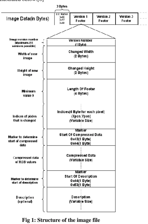
[image:1.595.329.566.381.738.2]The image file contains various components briefly illustrated below.[6]
Fig 1: Structure of the image file
2 Pixel information may be compressed depending upon the
image file format.
E.O.I.: This field is the marker representing end of the original image data. Its size is 3 bytes. When dealing with different image file formats, it can be a burdensome job to find the end of the image data with different header structures. In such cases, this field can be helpful to locate the end of image data. The values in these 3 bytes is static: 0x45, 0x4F, 0x49.
Version: The fields denoted as Version 1, Version 2, … are the footers attached to the original image file in order to represent various variations made to the file. Each of the these Versions follow a common structure described in the figure above. Version numbers serves as an id to different variations made. Size of Version number field is 1 byte.
Changed Width: This field indicates the new width of the image file. It represents the original width of the image when no additional pixels are added to the image. Size of Changed Width is 2 bytes.
Changed Height: This field indicates the new height of the image file. It represents the original height of the image when no additional pixels are added to the image. Size of the Changed Height is 2 bytes.
Footer Length: This field indicates the total size of the footer attached. Size of this is 4 bytes. Value of this field depends on the variable fields such as pixel indices and compressed data, description.
Pixel Indices: This field represents the indices of the pixels that are changed from the original image file. It occupies 4 bytes for each pixel. The overall size of this field depends on the number of pixels that are changed. The value of this field is the product of the pixel’s x- and y-positions.
Marker1: This field is the marker that represents the offset to the new data. The size of this field is 2 bytes.
Compressed Data: This field represents the compressed data of the RGB values using JPEG compression. These RGB values corresponds to the pixel defined by pixel indices. The size of this field depends on the number pixels changed.[2]
Marker2: This field is the marker that represents the offset to the description field. The size of this field is 2 bytes.
Description: This is the optional field. This field describes the message regarding to the change made to the original image, if any.
4.
WORKING
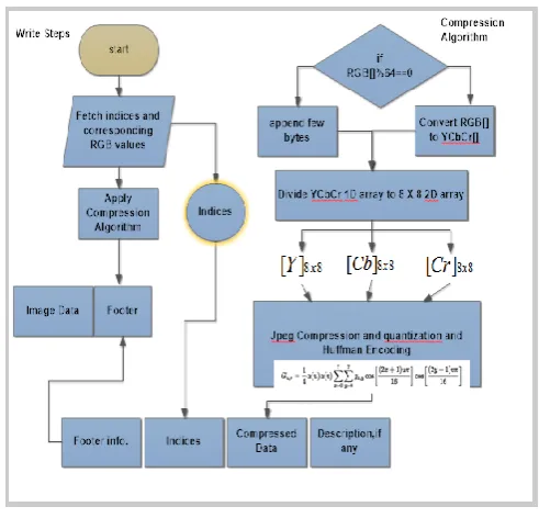
4.1 Write
This section comprises of compression of the data, footer formation and appending the footer to the original image. The primary steps associated with this section are as follows:
a) Selecting the old or new indices for the pixels that are to be changed or added respectively.[12] b) Deciding the RGB values for the above chosen
pixels.[11]
c) Applying the compression algorithm to the selected RGB values.
[image:2.595.311.557.69.305.2]d) Formation of the footer using various fields as discussed earlier and appending the footer to the original image data.[7]
Fig 2: Flowchart for Compression Algorithm
Compression Algorithm:
1. The new selected values are converted from RGB into a different color space called Y’CBCR. The Y’ component represents the brightness of a pixel, and the CB and CR components represents the chrominance split into blue and red components. Following equation converts the RGB values to Y'CBCR[5] .
Y′= 0.299R + 0.587G + 0.114B CB= −0.169R − 0.331G + 0.5B
CR= 0.5R − 0.419G − 0.081B
2. After the color space transformation, the Y’CBCR values are split into 8x8 blocks. If the data does not represent an integer number of blocks then the remaining area of the incomplete blocks are filled with some form of dummy data.
3.
Next, each 8x8 block of each component is converted to a frequency-domain representation, using a normalized Discrete Cosine Transform(DCT). Before computing the DCT of the 8x8 block, its values are shifted from a positive range to one centered on zero. For an 8-bit image, each entry in the original block falls in the range [0,255]. The midpoint of the range is subtracted from each entry to produce a data range that is centred on zero, so that the modified range is [-128,127]. The next step is to take the two dimensional DCT[4], which is given by:G
u,v=
14α u α v g
x,ycos
2x + 1 uπ
16
cos
2y + 1 vπ
16
7y=0 7
x=0
where,
u is the horizontal spatial frequency, for integers, 0 ≤ u ≤ 8
v is the vertical spatial frequency, for integers, 0 ≤ v ≤ 8.
α u = 1
√2, if u = 0
make the transformation orthonormal.
gx,y is the pixel value at coordinates x, y .
Gu,v is the DCT coefficient at coordinates u, v .
4. Next is dividing each component in 8x8 block by a constant for that component and then rounding to the nearest integer. This rounding operation is the only lossy operation in the whole process if the DCT computation is performed with sufficiently high precision. The elements in quantization matrix control the compression ratio, with larger values producing greater compression. A typical quantization matrix used is as follows:
Q
=
99
103
100
112
98
95
92
72
101
120
121
103
87
78
64
49
92
113
104
81
64
55
35
24
77
103
109
68
56
37
22
18
62
80
87
51
29
22
17
14
56
69
57
40
24
16
13
14
55
60
58
26
19
14
12
12
61
51
40
24
16
10
11
16
The quantized DCT coefficients[1] are computed with
Bj,k= round Gj,k Qj,k
for j = 0,1,2, … , 7; k = 0,1,2, … , 7
where G is the un quantized DCT coefficient; Q is the Quantization matrix above mentioned and B is the quantized DCT coefficients.
[image:3.595.312.557.349.609.2]
5. Next step is entropy coding, which involves arranging the image components in a ‘zigzag’ order employing run-length encoding (RLE) algorithm that groups similar frequencies together, inserting length coding zeros, and then using Huffman coding[8] on what is left. In N 8x8 blocks, if the ith block is represented by Bi and positions within each block are represented by p, q where p = 0,1, … ,7 and q = 0,1, … ,7 , then any coefficient in the DCT image can be represented as Bi p, q .
Fig 3: Zigzag ordering of image components
Thus, in the above fig 4.[1], the order of encoding pixels for the ith block is B
i 0,0 , Bi 0,1 , Bi 1,0 , Bi 2,0 , Bi 1,1 , Bi 0,2 , Bi 0,3 and so on. The process of encoding the zig-zag quantized data begins with a run-length encoding where:
x is the non-zero, quantized AC coefficient.
RUNLENGTH is the number of zeroes that came before this non-zero AC coefficient
SIZE is the number of bits required to represent x.
AMPLITUDE is the bit representation of x.
The run-length encoding works by examining each non-zero AC coefficient x and determining how many zeroes came before the previous AC coefficient[1]. With this information, two symbols are created:
Table 1. Huffman encoding
Symbol 1
Symbol 2
(RUNLENGTH,
SIZE)
(AMPLITUDE)
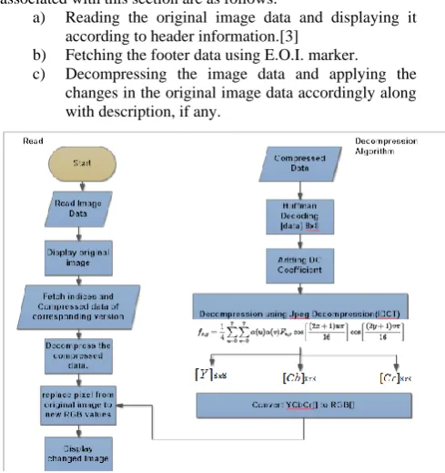
4.2 Read
This section comprises of displaying original image according to the header information, decompressing the footer and displaying the modified image accordingly. The primary steps associated with this section are as follows:
a) Reading the original image data and displaying it according to header information.[3]
b) Fetching the footer data using E.O.I. marker. c) Decompressing the image data and applying the
changes in the original image data accordingly along with description, if any.
Fig
4: Flowchart for Decompression AlgorithmDecompression Algorithm:
1. The compressed data is first processed through Huffman decoding in which the sequential data is transformed into 8x8 blocks using the above mentioned symbol table. These blocks are the quantized DCT[2] coefficient matrices.
[image:3.595.77.275.595.754.2]4 3. Now, the two dimensional inverse DCT[2] of the
resulting DCT coefficient matrices is taken which can be given by :
fx,y=1
4 α u α v Fu,vcos
2x + 1 uπ
16 cos
2y + 1 vπ 16 7
v=0 7
u=0
Where
x is the pixel row, for the integers 0 ≤ x ≤ 7.
y is the pixel column, for the integers 0 ≤ y ≤ 7.
α u is defined as above, for the integers 0 ≤ u ≤ 7.
Fu,v is the reconstructed approximate coefficient at coordinates u, v .
fx,y is the reconstructed pixel value at coordinates x, y .
Since, rounding the output to integer values results in an image with values still shifted down by 128, this value is added to each entry. In general, the decompression process may produce values outside the original input range of [0,255]. If this occurs, the decoder will clip the output values keeping them in that range to prevent overflow when storing the decompressed image with original bit depth.
4. Each of the resulting blocks of matrices represents values in one of the color space format namely: Y’ or CB or CR. Now these components need to be converted to RGB format based on following equations[5]:
R = Y′+ 1.402CR
G = Y′− 0.344CB− 0.714CR B = Y′+ 1.722CB
[image:4.595.335.547.70.425.2]The output from the above mentioned decompression steps gives the decompressed data which can be used to make change in the original image pixels[10] associated with the corresponding indices in the footer.
Fig 5: Original Image
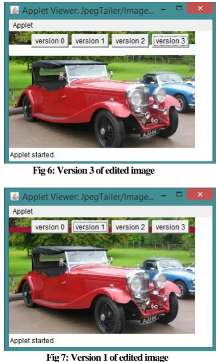
Fig 6: Version 3 of edited image
Fig 7: Version 1 of edited image
5.
CONCLUSION
In this paper, mechanism to store and retrieve partially changed image data are discussed along with the generalized structure of the file format which can be used with various base file formats such as JPG, PNG, GIF, etc. The logic to read appended versions and related information is discussed. Moreover the file format designed is in such a way that the modified file under version control system is still usable with standard viewer application. Along with storing version related data, an encryption technique is also discussed to secure the information.
Proposed file format, encryption technique[4] and read/write algorithms are useful in effectively managing multiple versions of a base image file having partial changes in it. By further developing this mechanism it can be implemented for processing the images captured by geostationary satellite.
6.
REFERENCES
[1] Jpeg n.d. In Wikipedia. Form https://en.wikipedia.org/wiki/JPEG
[2] Guocan Feng, Jianmin Jiang, JPEG compressed image retrieval via statistical features, Pattern Recognition, Volume 36, Issue 4, 2003, Pages 977-985, ISSN 0031-3203, http://dx.doi.org/10.1016/S0031-3203(02)00114-0.
[image:4.595.82.291.523.682.2][4] Krikor, Lala, et al. "Image encryption using DCT and stream cipher." European Journal of Scientific Research 32.1 (2009): 47-57.
[5] A. M. Sapkal, M. Munot and M. A. Joshi, "R'G'B' to Y'CbCr color space conversion Using FPGA," 2008 IET International Conference on Wireless, Mobile and Multimedia Networks, Beijing, 2008, pp. 255-258. doi: 10.1049/cp:20080191
[6] N. R. Rao and K. C. Sekharaiah, "Embedding version tag in software file deliverables before build release," 2015 4th International Conference on Reliability, Infocom Technologies and Optimization (ICRITO) (Trends and Future Directions), Noida, 2015, pp. 1-6. doi: 10.1109/ICRITO.2015.7359255
[7] J. R. da Silva Junior, T. Pacheco, E. Clua and L. Murta, "A GPU-based Architecture for Parallel Image-aware Version Control," 2012 16th European Conference on Software Maintenance and Reengineering, Szeged, 2012, pp. 191-200. doi: 10.1109/CSMR.2012.28
[8] P. G. Howard and J. S. Vitter, "Fast and efficient lossless image compression," [Proceedings] DCC `93: Data Compression Conference, Snowbird,UT,1993,pp.351-360. doi: 10.1109/DCC.1993.253114
[9] B. Luo, X. Zhang and Z. Tan, "Metadata Namespace Management of Distributed File System," 2015 14th International Symposium on Distributed Computing and Applications for Business Engineering and Science (DCABES), Guiyang, 2015, pp. 21-25. doi: 10.1109/DCABES.2015.13
[10] L. Bonanni, X. Xiao, M. Hockenberry, P. Subramani, H. Ishii, M. Seracini, and J. Schulze, "Wetpaint: scraping through multi-layered images," in Proceedings of the 27th international conference on Human factors in computing systems, ser. CHI '09. New York, NY, USA: ACM, 2009, pp. 571-574. [Online].
[11] J. Wong and M. A. M. Capretz, "An implementation for merging images for version control," in Proceedings of the 10th WSEAS international conference on Computers, ser. ICCOMP'06. Stevens Point, Wisconsin, USA: World Scientific and Engineering Academy and Society (WSEAS), 2006, pp. 662-667. [Online]. Available: http://portal.acm.org/citation.cfm?id=1981848.1981971