Factor regression for dimensionality reduction and data integration techniques with applications to cancer data

warwick.ac.uk/lib-publications

A Thesis Submitted for the Degree of PhD at the University of Warwick

Permanent WRAP URL:

http://wrap.warwick.ac.uk/130061

Copyright and reuse:

This thesis is made available online and is protected by original copyright.

Please scroll down to view the document itself.

Please refer to the repository record for this item for information to help you to cite it.

Our policy information is available from the repository home page.

dimensionality reduction and

data integration techniques

with applications to cancer data

Alejandra Avalos Pacheco

Thesis submitted for the degree ofDoctor of Philosophy

University of Warwick Department of Statistics

List of Figures vi

List of Tables x

List of Algorithms xii

Acknowledgements xvii

Declaration xix

Abstract 1

1 Introduction 3

1.1 Motivation . . . 3

1.2 Dimensionality Reduction . . . 5

1.2.1 Principal Component Analysis . . . 6

1.2.2 Probabilistic Principal Component Analysis . . . 7

1.2.3 Factor Analysis . . . 8

1.3 Sparsity . . . 10

1.4 Non-local priors . . . 11

1.5 Combining data and batch effects . . . 14

1.5.1 Data “normalisation” . . . 15

1.5.2 Matrix factorization-based methods . . . 15

1.5.3 Location-scale methods . . . 15

2 Bayesian factor analysis with a novel Spike-and-Slab prior 19 2.1 Introduction . . . 19

2.2 Bayesian factor analysis . . . 20

2.2.2 Prior formulation . . . 22

2.2.3 EM algorithm for factor analysis model under uniform p(M) . . . 23

2.3 Latent factor cardinalityq . . . 25

2.4 Spike-and-Slab prior . . . 25

2.5 Normal-spike-and-slab . . . 27

2.5.1 Formulation . . . 27

2.5.2 EM algorithm for Normal-SS . . . 27

2.6 Laplace-spike-and-slab . . . 30

2.6.1 Formulation . . . 30

2.6.2 EM algorithm for Laplace-SS . . . 30

2.7 Non-local priors . . . 32

2.8 Normal-spike-and-MOM-slab . . . 33

2.8.1 Formulation . . . 33

2.8.2 EM algorithm for MOM-SS . . . 34

2.9 Laplace-Spike-and-MOM-Slab . . . 36

2.9.1 Formulation . . . 36

2.9.2 EM algorithm for Laplace-MOM-SS . . . 38

2.10 Prior elicitation . . . 40

2.11 Initialisation of parameters . . . 41

2.12 Post-processing for model selection and dimensionality reduction . . . 42

2.13 Simulation studies . . . 44

2.13.1 Dense loadings . . . 46

2.13.2 Truly sparse loadings . . . 48

2.14 Conclusions . . . 50

3 Batch effect correction using Bayesian factor regression 51 3.1 Introduction . . . 51

3.2 Latent factor regression with batch effects . . . 52

3.3 Prior formulation . . . 53

3.4 Parameter estimation . . . 55

3.4.1 EM algorithm under a uniform prior . . . 55

3.4.2 EM algorithm for spike-and-slab priors . . . 58

3.4.3 Initialisation of parameters . . . 62

3.4.4 Post-processing for model selection, dimensionality reduction and normalised data visualisation . . . 63

3.5 Results . . . 63

3.5.2 Truly sparse loadings . . . 65

3.6 Discussion . . . 69

4 Applications to cancer data sets 71 4.1 Applications to public cancer data sets . . . 72

4.1.1 The Clinically Annotated Data for the Ovarian Cancer Transcrip-tome . . . 72

4.1.2 The Cancer Genome Atlas (TCGA): lung cancer . . . 76

4.2 Application to off the press Pancreatic Cancer dataset . . . 79

4.3 Discussion . . . 82

5 Extensions and future work 83 5.1 Different factors across batches . . . 83

5.2 Integrative model-based factor analysis . . . 85

5.3 Further extensions . . . 89

6 Discussion 91 Appendix 93 A Reproducibility: R package . . . 93

A.1 Getting started . . . 93

A.2 Bayesian factor analysis . . . 93

A.3 Bayesian factor regression . . . 95

A.4 Tables . . . 96

A.5 Plots . . . 97

A.6 Post-processing of the latent factors . . . 98

B Ovarian cancer unsupervised:Z₃vsZ₄latent factors . . . 99

C Lung cancer unsupervised:Z₃vsZ₄latent factors . . . 100

D Pancreatic cancer unsupervised:Z₃vsZ₄latent factors . . . 101

Glossary 102

Notation Glossary 105

1 Principal component analysis representation. . . 7

2 Local priors form_jk under a modelγ_jk =1. . . 11

3 Non-local priors form_jk under a modelγ_jk ,0. . . 12

4 DAG for Bayesian factor analysis for Flat loadings matrix. . . 23

5 Comparison of Beta 1 k,1at different values of k. . . 26

6 Directed acyclic graph (DAG) for Bayesian factor analysis with batch ef-fect correction for Spike-and-slab prior on the loadings matrix. . . 27

7 Maximisation ofm_jk for Laplace-SS. . . 32

8 Priors and inclusion probabilities for Normal-SS and MOM-SS . . . 33

9 Maximisingm_jk for MOM-SS. . . 36

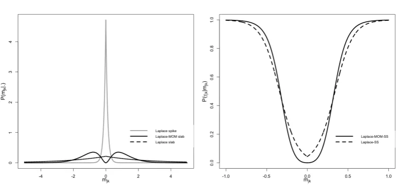
10 Priors and inclusion probabilities for Laplace-SS and Laplace-MOM-SS . . 37

11 Maximisingm_jk for Laplace-MOM-SS. . . 40

12 Comparison of the log-posterior convergence at different initialisations of parameters. . . 42

13 Left-ordered function for the latent indicators. . . 44

14 Heatmaps of data-generating loadings and covariance. . . 45

15 Scatterplots comparing true vs reconstructed factors and loadings in sim-ulations without batch effect and dense loadings. . . 46

16 Heatmaps of loadings and covariance for dense loadings scenario without batch effect. . . 47

17 Heatmaps of inclusion probability for dense loadings scenario without batch effect. . . 47

18 Scatterplots comparing true vs reconstructed factors and loadings in sim-ulations without batch effect and truly sparse loadings. . . 48

20 Heatmaps of inclusion probability for truly sparse loadings scenario with-out batch effect. . . 49

21 Directed acyclic graph (DAG) for Bayesian factor regression with Batch Effect correction. . . 54 22 Comparison of the log-posterior convergence at different initialisations of

parameters in scenarios with batch effect. . . 62 23 Scatterplots comparing true vs reconstructed factors and loadings in

sim-ulations with batch effect and dense loadings. . . 66 24 Heatmaps of loadings and covariance for dense loadings scenario with

batch effect. . . 66 25 Heatmaps of inclusion probability for dense loadings scenario with batch

effect. . . 66 26 Scatterplots comparing true vs reconstructed factors and loadings in

sim-ulations with batch effect and sparse loadings. . . 67 27 Heatmaps of loadings and covariance for truly sparse loadings scenario

with batch effect. . . 68 28 Heatmaps of inclusion probability for truly sparse loadings scenario with

batch effect. . . 68

29 Histogram of the gene expression variance across all samples forE.MTAB.386 andGSE30161ovarian cancer datasets. . . 73 30 First two factors of ovarian cancer datasets for the two different batches . 74 31 Histogram of the gene expression variance across all samples for theU133A

2.0andExon 1.0 STlung cancer datasets. . . 77 32 First two factors of lung datasets for the two different batches . . . 78 33 Histogram of the gene expression variance across all samples for

pancre-atic cancer dataset. . . 80 34 Heatmaps of reconstructed loadings and latent factors for pancreatic

can-cer datasets. . . 80 35 First two factors of pancreatic datasets for the two different batches. . . . 81

36 Directed acyclic graph (DAG) for Bayesian Factor Analysis with Batch Ef-fect correction and different factors per batch for Spike-and-slab loadings. 84 37 Group factor analysis. . . 86 38 Directed acyclic graph (DAG) for Bayesian factor regression with specific

39 Comparison of the log-likelihood convergence for Flat, Normal-SS, and MOM-SS priors for Bayesian factor regression with specific factors per data source model. Log-likelihood value at convergence for MOM-SS in dotted line. . . 89 40 Heatmaps for Bayesian factor regression with specific factors per data

source model. . . 90

1 Synthetic data without batch effects forn = 100,q∗ = 10,p = 1,000or 1,500parameters, dense loadingsM∗. . . 46

2 Synthetic data without batch effects forn = 100,q∗ = 10,p = 1,000or 1,500parameters, truly sparse loadingsM∗. . . 48

3 Synthetic data with batch effects forn = 200,q∗ = 10,p = 250or 500

parameters, dense loadingsM∗_{. . . 65}

4 Synthetic data with batch effects forn = 200,q∗ = 10,p = 250or 500

parameters, truly sparse loadingsM∗_{. . . 67}

5 Supervised analysis for gene expression of ovarian dataset (p=1,007genes). 76

6 Supervised analysis for gene expression of lung cancer dataset (p =1,198

genes). . . 77 7 Unsupervised analysis for pancreatic cancer dataset (p=1,177genes). . . 79

8 Cross-validated log-likelihood analysis for pancreatic cancer dataset (p=

1,177genes). . . 82

9 Synthetic data with batch effects and batch specific factors forn = 200,

q∗₌

1 EM algorithm for factor analysis model with uniform p(M) . . . 23

2 EM algorithm for factor analysis model with spike-and-slab p(M) . . . 28

3 Weighted 10-fold cross-validation for Bayesian factor analysis . . . 43

4 EM algorithm for factor regression model with uniform p(M) . . . 57

5 EM algorithm for factor regression model with spike-and-slab p(M) . . . . 59

Firstly I thank my supervisors, David Rossell and Richard Savage, who were always helpful, supportive, insightful and patient. I am deeply grateful to them for truly caring about my personal and professional development and well-being.

I also acknowledge David Firth and Francesco Stingo who carefully examined my the-sis and provided brilliant comments and useful suggestions. They let my viva be an en-joyable moment.

I would also express my gratitude to many other Warwick, Oxford and UPF scientist and faculty members for the enlightening discussions. I particularly thank Chris Yau for valuable insights and provided data.

I am grateful to all my Warwick and Oxford friends: it has been an honour to have them in my life. I especially thank the “team Savage”, who talked through ideas with me, and to Karla, Panayiota and Lewis: without them I would not have been able to submit this thesis (literally and figuratively).

Thanks to my family, in particular to my parents and papa Coco. Thanks for all the love and for always believing in me.

I declare that I have written and developed this PhD thesis entitled“Factor regres-sion for dimenregres-sionality reduction and data integration techniques with applica-tions to cancer data”completely by myself, under the supervision of Dr. David Rossell

and Dr. Richard S. Savage, for the degree of Doctor of Philosophy in Statistics. I have not used sources or means without declaration in the text. I also confirm that this thesis has not been submitted for a degree at any other university.

During my PhD I have written the article:“Heterogeneous large datasets integra-tion using Bayesian factor regression”(Avalos-Pacheco et al., 2018), in collaboration

with my supervisors Dr. David Rossell and Dr. Richard S. Savage. This article has been submitted to a peer reviewed journal and is still under revision. A preprint of this article can be found athttps://arxiv.org/abs/1810.09894

Introduction

1.1

Motivation

New technologies enable the gathering of large datasets. While these offer great promise for science, policy making and industry, their large volume and in particular the large number of recorded variables make its analysis and interpretation more challenging. Two main challenges in dealing with this high volume of data from a statistical per-spective are:

(i) Thehigh dimensional nature of the dataoften leads to models with a large number of parameters. These can be hard to handle, may obstruct interpretability, and often require computationally intensive calculations. A first important task when study-ing large datasets is to conduct an exploratory analysis: dimensionality reduction techniques have proven to be a highly popular tool for this purpose.

(ii) Batch effects, i.e. systematic biases in data that are unrelated to the scientific signal of interest, might arise when data are generated under different experimental condi-tions, when new samples are incrementally added to existing samples, or in analyses coming from different projects, laboratories, or platforms. Batch effects may lead to biased or inaccurate inference, unless properly adjusted for (Leek et al., 2010; Goh et al., 2017).

(i) A novel and scalable non-local prior based formulation to induce sparsity and learn the underlying number of factors, including important aspects related to prior elic-itation. To our knowledge this is the first adaptation of non-local priors to factor models.

(ii) A flexible model-based Bayesian factor regression approach for correcting batch ef-fects.

(iii) An efficient and scalable Expectation Maximisation algorithm with closed-form up-dates to obtain the Maximum A Posteriori (MAP) parameter estimates.

(iv) An R implementation publicly available athttps://github.com/AleAviP/BFR.BE.

(v) Application of these new methods to a variety of real-world and synthetic data sets.

As we will see, non-local priors provide a good balance between sparsity and sensitivity in inferring non-zero loadings; moreover, they give a better estimation of factor cardinality than other similar sparse inducing priors, even in scenarios without batch effects.

In this thesis we will focus on cancer-related gene expression data as our main moti-vating application. Cancer is one of the most studied pathological systems and one of the leading causes of morbidity and mortality worldwide. In 2012 about 14.1 million new cases occurred globally and about 8.2 million people died from cancer, corresponding to 14.6% of all human deaths (World Health Organization, 2014). It is expected that the number of annual cases will rise from 14 million in 2012 to 22 million within the next 20 years. Cancer cases occur more commonly in developed countries and risk increases significantly with age. In the UK, for example, more than one in three people will develop some form of can-cer during their lifetime (NHS, 2015); the survival rate is around 50%, and it is estimated that 42% of the cases could be prevented (Cancer Research UK, 2015).

Dimensionality reduction techniques are a popular tool for a better understanding of cancer (Gligorijevic and Przulj, 2015) and can lead to a more comprehensive analysis and easier interpretation of the data (Kristensen et al., 2014). On the other hand, batch effects are a major issue that arises in cancer datasets (Choi et al., 2017) and needs to be corrected in order to obtain accurate conclusions (Johnson and Li, 2009; Zhu et al., 2017).

Let us also notice that batch effects are present in many other research fields, such as structural magnetic resonance imaging (MRI) data from Alzheimer’s disease (Shinohara et al., 2014; Fortin et al., 2016), multiple sclerosis (Shah et al., 2011), and attention deficit hyperactivity disorder (Olivetti et al., 2012), or even toxicological studies in marine species (Avio et al., 2015).

and batch effect correction techniques: we present the current state-of-the-art and pro-vide the necessary background for our model.

1.2

Dimensionality Reduction

Dimensionality reduction techniques represent the data into a low-dimensional Eu-clidean space that gives insight into its underlying structure in order to visualise, denoise or extract meaningful features.

LetX ∈ ’n×p be a data matrix, where entryx_ij is theithobservation corresponding

to thejthvariable (i=1, . . . ,n andj =1, . . . ,p) andxT_i denotes theithrow. We will refer

toX as the high-dimensional matrix, alluding to the fact that the number of variablesp

is potentially large. Without loss of generality, it will be assumed from now on thatX has zero column means. LetZ ∈’n×q be a low-dimensional matrix (in the sense thatqp), withzTi denoting theithrow.

The goal of dimensionality reduction methods is, given X ∈ ’n×p, to obtainZ ∈

’n×q (q p) that in some respect provides a useful and more compact representation of the original data. This is done by finding a functionZ = f(X), requiring that the low-dimensional representation possesses some desirable properties, such as preserving variance or capturing covariance. Typically, given a pre-specified class of functionsF, one searches for a function f that achieves

min

f∈ Fд(X,f(X)) (1.1)

whereд(·)measures the quality of the low-dimensional representation. We remark that

дmight be some distance or discrepancy measure, as in the classical optimisation-based approaches to dimensionality reduction, but can also arise from a likelihood or posterior density function in model-based frameworks.

1.2.1 Principal Component Analysis

Principal Component Analysis (PCA) is a linear dimensionality reduction technique developed by Pearson (1901) to transform the high-dimensional dataX into a low-dimen-sional representationZ, such thatZ is a linear uncorrelated transformation of X that conserves as much variance as possible.

PCA minimises the reconstruction error via least squares optimisation:

min||X −ZM>||2

subject toM>_{M =I,} (1.2)

withM ∈’p×q,q ≤p.

Equation (1.2) is optimised when

b

Z =XMb(Mb

>

b

M)−1=XMb. (1.3)

We are left to find the matrixM. The optimal solution to (1.2) is obtained via the Singular Value Decomposition (SVD) ofX:

X =U LV> _(1.4)

whereU, called left singular vectors, is ann×n orthogonal matrix(U>U = I);V, called right singular vectors, is ap×porthogonal matrix(V>V = I)andL is ann×pdiagonal matrix with non-negative real diagonal entries called singular valuesλ₁ ≥ λ₂ ≥ · · · ≥

λ_min(n,p) ≥0. In terms of this factorisation, the covariance matrix

Σ=X>_{X =V L}2_V> _(1.5)

has the same right singular vectorsV asX. Using the SVD, we have thatZ =U L1/2_and M =L1/2_V>_{, and}

b

M =V_qL1/2

q (1.6)

gives the rankqsolution, whereA_qare the firstqcolumns of a given matrixA,V_q contains theqeigenvectors (called singular vectors) corresponding to the largest eigenvalues, and

b

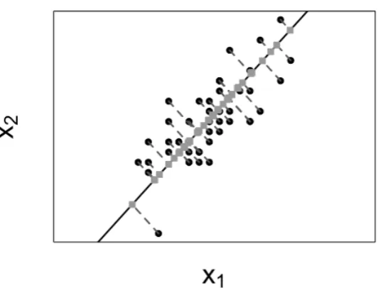
Figure 1. Principal component analysis representation: 2-dimensional vari-ablesX in black points and 1-dimensional representationsZ in squared grey points.

1.2.2 Probabilistic Principal Component Analysis

Probabilistic Principal Component Analysis (PPCA) (Tipping and Bishop, 1999) adds a probabilistic generative model to PCA. ObservationsX are seen as linear combinations of principal componentsZ plus ann×pmatrix of errorsE, wheree>_i denotes theithrow ande_ij ∼N(0,σε2)are independent acrossi =1, . . . ,n,j =1, . . . ,p:

xi =Mzi+ei. (1.7)

Note that PPCA assumes the variance to be constant across(i,j): this assumption is re-laxed by factor models by allowing sigma to depend onj.

The low-dimensional representations are independent standard normal random vari-ableszi ∼N(0,Iq), fori=1, . . . ,n.

model p(x_i |M,σ_ε)=N(0,MM>+σε2Ip), leading to the log-likelihood:

logp(x_i |M,σ_ε) ∝ −1

2

n

Õ

i=1

x>

i (MM>+σε2I)−1xi−n

2log|MM

>_+σ2

εI|. (1.8)

Notably Equation (1.8) can be maximised in closed-form. Specifically, maximisation with respect toM gives

b

M =V_q(L_q −σ_ε2I)1/2, (1.9) wherebΣ= _n1X

>_{X =V}>_L2_{V is the SVD, and the maximum likelihood estimator forσ}2

ε is

b

σ2

ε = _(p−1_q) p

Õ

j=q+1

λ_j. (1.10)

We note that p(z_i | x_i,M,σ_ε)=N((M>M+σ_ε2Iq)−1M>xi,σε2(M>M+σε2Iq)−1). Thus,

E[zi |xi,Mb,_bσε]=(Mb

>

b

M+bσ 2

εIq)−1Mb

>_x

i

=(I_q +_bσ_ε2I_q)−1Mb

>_x

i,

(1.11)

sinceMTM =I.

Then, PPCA can be seen as a ridge-type regression ofzi versusxi with penaltyσε2, recovering PCA whenσ2

ε is zero.

Extensions of this method include Ulfarsson and Solo (2008), who added a Gaussian shrinkage priorp(M)on the entries ofM, and Kao and Roy (2013), who imposed shrinkage by a penalty on the inverse covariance matrix.

1.2.3 Factor Analysis

Factor analysis is a dimensionality reduction technique that aims to describe the co-variance of an observed set of variables. It was originally introduced by Spearman (1904) as a tool for psychometric analysis. The observed variables xi ∈ ’p,i = 1, . . . ,n, are modelled as in (1.7), but hereei are independent Gaussianei ∼ N(0,T−1), whereT is a

p×pdiagonal matrix,z_i ande_i are independent,z_i ∼ N(0,I_q). In this context variables, zi are called latent factors,M ∈ ’p×q is the matrix of factor loadings, andT−1are the idiosyncratic variances (Fruchter, 1955).

distribu-tion ofxi isxi |M,T ∼N(0,MM>+T−1). Hence, the log-likelihood is:

logp(X |M,T ) ∝ −1

2

n

Õ

i=1

x>

i (MM>+T−1)−1xi −n₂log|MM>+T−1|. (1.12) The conditional distribution of the latent factors is

zi | xi,M,T ∼N((M>T−1M+Iq)−1M>Txi,(M>T−1M+Iq)−1). (1.13)

Thus, conditional on some estimated(Mb,T )b , a simple option to obtain low-dimensional coordinates is to use

E[zi | xi,Mb,T ]b =(Mb

>

b

T−1Mb+Iq)

−1 b

M>

b

Tx_i. (1.14)

However, obtaining (Mb,T )b via MLE or posterior mode estimation cannot be done in closed-form as in PPCA, hence a numerical optimisation scheme such as the Expectation-Maximisation algorithm is used to estimate them.

Notice that, when the observation noise isT−1=σ_ε2I, we recover PPCA, whereas for T−1=0we obtain PCA. Thus, we will focus on FA for the sake of generality.

1.3

Sparsity

From a statistical point of view it is often desirable to enforce sparse solutions to improve interpretability and, when the number of parameters to be estimated is large, potentially also improve the accuracy of statistical inference. Moreover we argue that, as an additional motivation, sparsity is a bona-fide prior expectation in certain applications. For instance, in genetics a few active genes could potentially explain a whole complex biological system; e.g. it was found that few latent variables associated to the cerebrum tissue of mice could be used to provide their genomic “true age” (Perry and Owen, 2010). In psychology, some social behaviours could be explained via latent factors: four of them were found to explain 81% of the total variance in a job scoring (Kendall, 1975). In social media, for example, the most popular videos played in YouTube were produced by 10,000 out of 1 billion users (Earnshaw, 2017).

Several strategies have been developed for sparse models, such as Least Absolute Shrinkage and Selection Operator (LASSO) regression (Tibshirani, 1994), Strawderman - Berger priors (Strawderman, 1971; Berger, 1980), nonconcave penalties e.g. smoothly clipped absolute deviation (SCAD) penalty (Fan and Li, 2001) or minimax concave penalty (MCP) (Zhang, 2010), and Horseshoe priors (Carvalho et al., 2009). Another approach is to model the loadings via spike-and-slab priors (SS), which are a mixture of two dis-tributions: one for the important loadings (slab) and another one for the non-important loadings (spike). One possibility is to model the spike component with a finite point mass on zero and the slab with a continuous density (Mitchell and Beauchamp, 1988; West, 2003; Knowles and Ghahramani, 2011).

In this thesis we focus on continuous SS models, estimating them via Expectation-Maximisation (EM) algorithms, which induce posterior zeroes on the loadings with high probability. As a starting point, we take the EM algorithm developed in Roˇckov´a and George (2017). The continuity of the spike distribution enables us to obtain closed-form expressions for the EM updates, providing a rapidly computable and scalable EM algo-rithm.

Letγ_jk ∈ {0,1} be latent indicators forj = 1, . . . ,p andk = 1, . . . ,q, withγjk = 1 if latent factorz_jk is included in the model. In the SS models, the inclusion of the latent factorsz_jk is modelled through the loadingsm_jk. Thus, whenm_jk = 0, we setz_jk = 0,

distinguishing the latent factors to be excluded from the ones to be included. The loadings are modelled as follows:

whereλ₀andλ₁are the dispersion parameters of the spike and slab components respec-tively, withλ₁>λ₀.

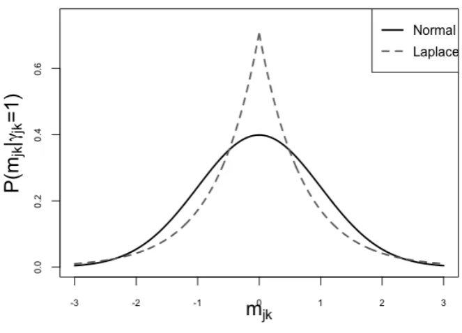
Figure 2.Local priors formjkunder a modelγjk =1.

Two popular densities in SS models for modelling the non-zero loadings are Normal (George and McCulloch, 1993) and Laplace (Roˇckov´a and George, 2018). Figure 2 shows the slab priors used to model the non-zero loadings therein. Notice that the regions of the real line to which the spike and the slab assign positive non-negligible probability “overlap” in a neighbourhood aroundm_jk = 0: thus, as we will see later (Figures 8 and

10 right panels), it becomes hard to tell which of them (spike or slab) generatedm_jk. To solve these issues, we then model the non-zero loadings with non-local priors.

1.4

Non-local priors

setting because, when modelling the non-zero loadings, they vanish asm_jk gets close to zero. In this context, any other prior that does not vanish asm_jk →0is called Local Prior

(LP).

We would like to model the probability p(m_jk | γ_jk = 0) for non-important loadings (m_jk =0) and the probability p(m_jk |γ_jk =1)for important loadings (m_{jk ,}0).

An NLP density can always be expressed as

p(m_jk |γ_jk =1)=d(m_jk)p_L(m_jk |γ_jk =1), (1.16) whered(m_jk)is a penalty term and p_L(m_jk |γ_jk =1)is a base local prior density (Rossell and Telesca, 2017).

Some default additive NLPs are:

Figure 3.Non-local priors form_jkunder a modelγ_jk ,0.

(i) Moment (MOM)(Johnson and Rossell, 2010). These priors are obtained as the

density pL(mjk)with2κ finite integer moments. The MOM density is then pM(mjk)=

m2κ

jk

ϒ pL(mjk), (1.17)

where

ϒ=

∫

m2κ

jkpL(mjk)dmjk

is called prior dispersion parameter. Under some conditions, MOM priors lead to closed-form expressions for MCMC algorithms and, as we will see in Chapter 2, for EM algorithms.

In this thesis, we consider the base local prior densities pL(mjk)to be either Normal or Laplace. The resulting MOM densities are the Normal-based prior:

m2

jk

e

λ₁ N(mjk; 0,eλ1), (1.18)

withϒ=eλ₁, and the Laplace-based prior:

m2

jk

2eλ2₁

Laplace(m_jk; 0,eλ₁), (1.19) withϒ=2λe2₁.

(ii) Inverse moment (iMOM)(Johnson and Rossell, 2010). iMOM densities are of the

form

pI(mjk)=

κeλϖ

/2 1

Γ(ϖ/2κ)

m2

jk

−(ϖ+1)/2

exp " − m 2 jk e λ₁

!−κ#

, (1.20)

forϖ,eλ₁>0. An iMOM prior has a similar form as an Inverse Gamma whenmjk →0. As we can see in Figure 3, the iMOM prior approaches zero faster than the MOM prior. The drawback of iMOM priors is that they do not lead to closed-form expressions for MCMC and EM algorithms.

(iii) Exponential Moment (eMOM)(Rossell et al., 2013). eMOM priors are

pE(mjk |γjk =1)=e

√ 2_exp

" − eλ1

m2κ

jk

#

eMOM priors is that the former vanish at a polynomial speed asm_jk →0, whereas

the latter vanish exponentially fast. In our experience MOM priors lead to simpler computation and, provided the prior parameters are suitably elicited, are enough to induce sufficient sparsity.

As a brief review, NLPs have been applied to Bayesian model selection (BMS) and model averaging (BMA) in linear regression (Johnson and Rossell, 2010, 2012; Rossell and Telesca, 2017); in some generalised linear models (Johnson and Rossell, 2012; Rossell et al., 2013); under orthogonal and block-diagonal regression (Papaspiliopoulos and Rossell, 2017); for mixture models (F´uquene et al., 2018); in linear regression with non-normal residuals (Rossell and Rubio, 2018). Finally, see Shi et al. (2018) for a more recent work in parallel that also applies Spike-and-slab priors with a MOM slab component for BMS in linear regression via Gibbs sampling. Outside the generalised linear model framework, NLPs have been also studied for directed acyclic graphs (Consonni and La Rocca, 2011), gene regulatory networks (Chekouo et al., 2015), chain event graphs (Collazo and Smith, 2016), and Bayesian graphical regression (Ni et al., 2018). In Chapter 2 we study Normal-based MOM priors in the FA setting, but we also discuss some Laplace-tailed extensions. To our knowledge this is the first adaptation of NLPs to factor models. As we will discuss later, the main advantage of NLPs in this setting is to help achieve a better balance between sparsity and sensitivity in inferring non-zero loadings.

1.5

Combining data and batch effects

When data from multiple sources, projects or experiments are available, one would like to perform a statistical analysis that incorporates all available information. In this setting it is important to take into account batch effects, i.e. systematic artefacts that may lead to imprecise or erroneous findings. Several batch effect correction algorithms (BECA) have been developed (see Scherer (2009); Lazar et al. (2013) for a review and examples). They can be divided into data “normalisation”, matrix factorisation-based and location-scale methods. We overview some popular strategies and discuss their advantages and limitations.

1.5.1 Data “normalisation”

The main idea behind data “normalisation” is to use control metrics or regression methods to correct for the high variability due to systematic noise and artefacts.

Linear normalisation is one of the most in demand algorithm, among data normali-sation BECA. Its main assumption is that the different observationsxi ∈ ’p are related linearly with a baseline experimentex∈’

p_{, as a straight line with a zero y-intercept. The}

method simply linear regressesexonxi, obtaining a scaling factorβ (slope of the line):

ex≈βxi. (1.22)

Other data normalisation algorithms include non-linear normalisation. See Schadt et al. (2001); Yang et al. (2002) for a review of data normalisation BECA.

“Normalisation” methods are useful but could fail when the variation between batches is large (Johnson and Li, 2009).

1.5.2 Matrix factorization-based methods

Matrix factorization-based BECA are grounded on the assumption that the most im-portant source of variability is associated with batches. Batch effect correction is per-formed in two steps:

(i) concatenate the data and perform a matrix factorization;

(ii) remove the factors associated with the batches and reconstruct the data.

Alter et al. (2000); Leek and Storey (2007) proposed an adjustment using singular value decomposition, and Benito et al. (2004) via distance weighted discrimination.

These approaches present some disadvantages. It might not be straightforward to identify the batch effect component, which can be confounded with other sources of vari-ance. Furthermore, these methods could potentially fail in cases where batches have small sample sizes or in the presence of many more than three batches (Johnson and Li, 2009).

1.5.3 Location-scale methods

Location-scale (LS) methods aim to standardise the data so that each batch displays the same or similar mean and/or variance per gene. We outline some of the most popular LS tools.

Letx_ijbe the observed data of individuali=1, . . . ,nfor variablej =1, . . . ,p. Assume

there aren_l individuals in batchl, so thatn =n₁+· · ·+n_p

b. Letbibe the indicator vector

Batch-mean centring

This method performs a mean batch correction only (Sims et al., 2008). It obtains a new corrected observationbxij such that

b

x_ij =x_ij−x¯_jl, (1.23)

wherex¯_jl = _n1

l

Ín

i=1xijbil is the sample mean of variablejin batchl.

Ratio-based methods

These methods are a straightforward extension of batch-mean centring. They subtract the geometric mean per batch, which is less sensitive to outliers (Novoradovskaya et al., 2004), instead of the sample mean:

b

x_ij =x_ij− nl v t n

Ö

i=1

x_ijb_il. (1.24)

The median or arithmetic mean ratio can be also used instead.

Data standardisation

Li and Wong (2001) consider that batches may affect not only means but also vari-ances. They therefore propose normalising the data to zero mean and unit variance per batch :

b

x_ij = xij−x¯jl

b

σ_jl , (1.25)

wherebσ 2

jl = n1l

Ín

i=1(xijbil −x¯jl)2is the estimated variance of variablejin batchl.

Regression-based LS adjustments

These BECA aim to mean center and standardise the variance for each variable per batch independently via a linear regression model:

x_ij =α_j +β>

j bi+δj>biεij, (1.26)

whereα_j is the overall intercept,β_j ∈ ’pb andδ

Some recent LS methods are the ones proposed by Leek and Storey (2007); Parker et al. (2014); Hornung et al. (2016). A more general approach, developed by Li and Wong (2003), consists in incorporating covariatesvi ∈’pv of interest. Here data are modelled as

x_ij =α_j +θ>

j vi+βj>bi+δj>biεij, (1.27)

withθ_j ∈ ’pv the regression coefficients. These covariates help to incorporate useful

information about the data (e.g. standard medical history) and to combine data from more diverse data sources (e.g. different platforms). The corrected data are

b

x_ij = xij−αbj −θb

>

j vi−βb>_j b_i

b

δ>

j bi

+αbj +θb

>

j vi, (1.28)

withαb,βb,θb,bδ the estimators forα,β,θ,δ.

Empirical Bayes: ComBat

The previous BECA are useful, but require that the sample size is large enough so that (α,θ,β)and particularly the variance batch effectδ2are estimated precisely. Johnson and Li (2009) proposed a method, called empirical Bayes batch effect correction (ComBat), which considers the model in (1.27), correcting the data via three steps:

(i) Data standardisation. Mean and variance variable-wise data standardisation of the

form:

y_ij = xij−αbj −θb

>

j vi

b

σ_j , (1.29)

using the least squares estimates.

(ii) Empirical Bayes parameter estimation. The standardised variables are assumed

to be distributed asy_ij ∼N(β_jl,δ_jl2), forb_jl =1. The prior specification is completed

withβ_jl ∼ N(µ_j,τ_j2) and δ_jl2 ∼ Inverse Gamma(λ_j,β_j). Such priors were selected due to their conjugacy. Hyperparametersµ_j,τ2

j,λj,βj are estimated empirically, and estimators forβ_jl andδ2

jl are obtained by their conditional posterior means.

(iii) Data correction. Data are corrected using the estimations obtained in Step (ii):

b

x_ij = bσj b

δ>

j bi

(y_ij−βb

>

jbi)+αbj +θb

>

j vi. (1.30)

sample sizes, improves precision, and avoids over-correcting the data. These are due to the fact that it uses empirical Bayes estimates and a hierarchical model, which borrows strength in the estimation ofδ across batches. Due to these advantages, we will compare our models with ComBat throughout this thesis.

Outline of the thesis. Chapter 2 reviews the Bayesian factor analysis model and

Bayesian factor analysis with a novel

Spike-and-Slab prior

2.1

Introduction

In this chapter we study dimensionality reduction via Bayesian factor analysis. Factor analysis had proven to be an efficient tool to obtain low-dimensional latent representa-tions of the high-dimensional data by extracting latent variables (or factors) from the data. Such factors aim to provide a better understanding of the complex data, generat-ing visual representations, new meangenerat-ingful features extracted from the data or denoised latent variables.

We present a novel type of continuous spike-and-non-local-slab prior to estimate the latent cardinality (number of factors). Those priors are based on Johnson and Rossell (2010, 2012) and on the continuous Gaussian spike-and-slab prior of George and McCul-loch (1997); Roˇckov´a and George (2014) and its Laplace-based extention (Roˇckov´a and George, 2017, 2018).

We provide an Expectation-Maximisation (EM) algorithm to obtain the Maximum A posteriori (MAP) estimation of the parameters. We provide closed-form EM updates, giv-ing a novel scalable algorithm for non-local priors. To our knowledge this is the first time non-local priors are implemented in factor analysis settings.

As we will discuss later, the main advantage of non-local priors in this setting is to help achieve a better balance between sparsity and sensitivity in inferring non-zero loadings. See also Bar et al. (2018) who argued for improved sensitivity via 3-component mixture priors that resemble non-local priors in generalised linear models.

for Normal-spike-and-slab priors and Section 2.6 for Laplace-spike-and-slab. Section 2.7 introduces non-local priors in the factor analysis context. Sections 2.8 and 2.9 provide our novel EM algorithms for our novel Normal-spike-and-MOM-slab and Laplace-spike-and-MOM-slab respectively. Section 2.10 provides guidelines for the prior elicitation. tion 2.11 and 2.12 discuss the initialisation and post-processing of the parameters. Sec-tion 2.13 shows the potential of our model with simulated data. Finally SecSec-tion 2.14 con-cludes. For the benefit of the readers already familiar with factor regression, we remark that our key methodological contributions are in Sections 2.7 - 2.12.

2.2

Bayesian factor analysis

Factor analysis (FA) models describe the observationsxi = (xi1,xi2, . . . ,xip) >

∈ ’p,

fori = 1, . . . ,n individuals as a regression over latent variables z_i ∈ ’q, called latent

coordinates or factors. Those latent coordinates tend to have a low-dimensionq p, making them easier to interpret and visualise. LetX be then×pmatrix with theithrow equal tox>

i andZ then ×q matrix of latent coordinates, containing z>i in theith row. More formally, the factor analysis model is defined as

xi =Mzi+ei, (2.1)

whereM ∈’p×q is the matrix of factor loadings ande_i ∈’p is the error, distributed as

ei ∼ N(0,T−1)independently acrossi = 1, . . . ,n, withT−1a diagonal matrix. Factors are assumed to be standard normal,zi ∼N(0,I), independent acrossi=1, . . . ,nand also independent ofei.

Without lost of generality, we have assumed that observationsxi have been mean centred, through this thesis. The non-centred model

xi =µ+Mzi+ei (2.2)

withµ ∈’p, can be seen as the centred model_ex_i =Mz_i+e_iwith_ex=x_i−µand estimating the mean with the sample meanbµ =X¯ =

1

nÍni xi.

Alternatively, Equation (2.1) can be given in matrix notation as

X =ZM>_{+E, (2.3)}

withE n×pmatrix of errors, containinge_i>in theithrow.

Integrating out the factors, the implied marginal density of xi is f(xi | M,T ) =

be decomposed with at mostpq+pparameters instead ofp+p(p−1)/2=p(p+1)/2.

The factor model is non-identifiable up to orthogonal transformations, of the form

M∗> _{= A}>_M>_andZ∗ _{=ZA, whereAis any orthogonalq}

×qmatrix. That is, the factor model in (2.3) can equivalently be rewritten as

X =Z∗_M∗>_{+E. (2.4)}

Clearly, both factor models generate the same covariance structure

Cov[x_i | M,T,A]=MM>+T−1=MAA>M>+T−1=M∗M∗>+T−1 (2.5)

To obtain unique point estimates ofMandZ, several strategies have been developed. One option is restricting the parameter space. Seber (1984) constrainedMsuch thatM>_AA>_M

is diagonal. Lopes and West (2004) restrictedMto be lower-triangular with a strictly posi-tive diagonal,m_{j j} >0, and assumedMto be full-rank. More recently, Fr¨uhwirth-Schnatter

and Lopes (2018) suggested a factor reordering via a Generalized Lower Triangular loading matrix. However, under this approach the interpretation ofM depends on the arbitrary ordering of the columns inX, and it gives special roles to the first factors. Another option is to encourage sparsity inM, e.g. the classical varimax solution (Kaiser, 1958) maximises the variance in the squared rotated loadings. A more modern strategy is to favour sparse solutions containing exact zero loadings, e.g. Roˇckov´a and George (2017) proposed an EM algorithm that seeks rotations based on a so-called Parameter Expansion that aims to avoid local suboptimal regions. We adopt a similar strategy where sparse solutions are preferred by the introduced non-local penalties. This prior formulation will be discussed in Section 2.4.

2.2.1 Inference methods

Several parameter estimation methods have been developed by others to infer the loadingsMand precisionT. We outline the principal component solution of factor anal-ysis and the Maximum likelihood methods; in subsequent sections we discuss Bayesian solutions

Principal component solution of factor analysis

At the core of this method is the fact that, given the number of latent factorsq, the sample covariance matrixS = 1

nX>X can be approximated by

1

nX >_X

≈MbMb

>

+Tb

Thus, the estimation ofMandT is given by the following two-step approach:

Step 1: Consider the eigendecomposition of _n1X>X wherel₁ ≤ l₂ ≤ · · · ≤l_q are the eigenvalues andu₁, . . . ,u_q are the eigen vectors. Then set

b

M =[pl₁u₁, . . . q

l_qu_q]. (2.7)

Step 2:Typically one takes the precision as

bτ

−1

j j =max{0,Sj j −mb

>

jmbj}. (2.8)

whereS = 1

nX>X andSj j its(j,j)element.

Maximum likelihood method

Recall thatxi | M,T ∼N(0,MM>+T−1). We then aim to maximise the log-likelihood

logp(X |M,T ) ∝ −1

2

n

Õ

i=1

x>

i(MM>+T−1)−1xi −n₂log|MM>+T−1|. (2.9) The estimators ofMbandTb

−1_{do not have a closed form, hence a numerical optimisation}

scheme – often Expectation-Maximisation (EM, Dempster et al. (1977)) – is normally used to obtain them. When incorporating priors to the FA model and performing posterior inference, one might also use EM algorithms, which give posterior modes. In addition to EM, estimation can also be carried out via MCMC algorithms (Lopes and West, 2004) to obtain the full posterior, or approximated via variational inference (Ghahramani and Beal, 2000). In this thesis we will provide deterministic optimisations to maximise the log-posterior via an Expectation-Maximisation algorithm that proved to be computationally efficient.

2.2.2 Prior formulation

To complete the Bayesian model specification we set some priors. As a first step we consider an improper flat prior on the loadings

p(M) ∝1. (2.10)

An obvious limitation of (2.10) is that it does not induce any shrinkage or sparsity, we defer such extensions to Section 2.4.

assume independent gamma priors

τ_j ∼Gamma(η/2,ηξ/2) (2.11)

j =1, . . . ,p. By default we setη=ξ =1, this choice of hyper-parameters lead to relatively

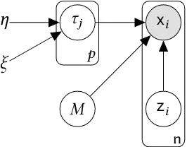
diffuse but proper priors. Figure 4 provides a Directed acyclic graph (DAG) for our model.

x

z

M

τ

η

ξ

Figure 4.DAG for Bayesian factor analysis for Flat loadings matrix.

2.2.3 EM algorithm for factor analysis model under uniformp(M)

The Expectation-Maximisation (EM) algorithm aims to maximise the log-posterior

logp(M,T | X) by working with the complete-data log-posterior logp(M,T | X,Z). This algorithm has two steps: the E-step calculates the expected log-likelihood w.r.t p(Z |

b

M,Tb,X), whereMband Tb are the current values of M and T. The M-step maximises

E[logp(M,T |X,Z)]w.r.t.MandT giving a new update for them.

To ease the notation, letb∆=(Mb,T )b be the current values ofMandT

Algorithm 1:EM algorithm for factor analysis model with uniform p(M)

initialiseMb=M

(0)_,

b T =T(0)

whileε >ε∗,ε_M >ε∗_M andt <T do E-step:

Latent factors: E[zi|b∆,X]=(Iq +Mb

>

b TMb)

−1 b

M>

b Tx_i

M-step:

Loadings: Mb= h

Ín

i=1xiE[z >

i | b∆,X] i h

Ín

i=1E[ziz >

i |b∆,X] i−1

Variances: Tb

−1₌ 1

n+η−2diag n

Ín

i=1

xix>i −xiE[zi |b∆,X]

>

b

M>

+ηξI_p

o

set∆(t+1)=b∆andM

(t+1)₌

b

M

computeε =Q(∆t+1) −Q(∆t),ε_M =max_j,k ||m(_jkt+1)−m(_jkt)||andt =t+1

The E-steptakes the expectation

Q(∆)=_EZ|

b∆,X[logp(M,T |X,Z)] ∝EZ|b∆,X [logp(X,Z | M,T )+logp(M,T )] ∝ − 1

2

n

Õ

i=1

E_Z|b∆,X

(x_i−Mz_i)>T (x_i−Mz_i) +n

2log|T |

+

p

Õ

j=1 η

−2

2 log(τj) −

ηξ

2 Tj

=− 1

2

n

Õ

i=1

EZ|b∆,X

x>

iTxi−2xiTMzi +z>iM>TMzi

+n+η−2

2 loд|T | −

ηξ

2 tr(T )

=− 1

2

n

Õ

i=1 h

x>

i Txi−2xiTME[zi |b∆,X]+tr(M

>

TM_E[z_iz>_i |b∆,X]) i

+n+η−2

2 loд|T | −

ηξ

2 tr(T ),

(2.12)

wheretr(A)is the trace of matrixA.

Note that Expression (2.12) only depends onZ through the conditional posterior mean

E[zi |b∆,X]=(Iq +Mb

>

b TMb)

−1 b

M>

b

Tx_i (2.13)

and the conditional second moments

E[zizi>|b∆,X]=(Iq +Mb

>

b TMb)

−1₊

E[zi |b∆,X]E[zi |b∆,X]

>_{. (2.14)}

The M-stepconsists in maximising Equation (2.12) with respect to∆. To this end, we

set its partial derivatives to 0, as shown below.

∂Q

∂M =−

1 2

n

Õ

i=1 h

−2TbxiE[z

>

i | b∆,X]+2TbMbE[ziz

>

i |b∆,X] i

=0 (2.15)

The maximum of the loadingsM can be found solving (2.15) as:

b

M =

" _n Õ

i=1

xiE[z>i |b∆,X] # " _n

Õ

i=1

E[ziz>i | b∆,X] #−1

Analogously, maximisation ofT is obtained by taking the derivative

∂Q

∂T =−

1 2

n

Õ

i=1 h

xix>i −2xiE[zi | b∆,X]

>

b

M>₊

b

ME[ziz>i |b∆,X]Mb

>i

+n+η−2

2 Tb

−1

−ηξ

2 Ip =0.

(2.17)

Substituting Equation (2.15) and using the diagonal constraint we obtain:

b

T−1= 1

n+η−2diag

( n Õ

i=1

xix>i −xiE[zi |b∆,X]

>

b

M>_+ηξ

I_p

)

(2.18)

Algorithm 1 summarises the EM algorithm. The stopping criterion is reaching a tol-eranceε∗_{in the log-posterior change, a maximum number of iterationsT or a changeε}∗

M on the loadings. By default we setε∗₌

0.001,T = 100andε∗_M =0.05. The EM algorithm

increases the complete-data log-posterior at each iteration, however it does not guaran-tee convergence to a global maximum. Thus, initial values are crucial in order to obtain a good performance. Parameter initialisation is discussed in Section 2.11.

2.3

Latent factor cardinality

q

The choice of the cardinality of the latent factorsqis a crucial aspect in FA. Until now

qwas assumed known. In practice, there are several strategies to inferq. One option is to treat the problem as a model selection, choosingqwith the smallest Akaike information criterion (AIC) or Bayesian information criterion (BIC). Another option is to consider a single model with largeqand set penalties or priors that induce sparse solutions, where only some small proportion of the loadings are non-zero, easing the interpretation of the model. Some recent strategies include a LASSO-based method (Witten et al., 2009), horse-shoe priors (Carvalho et al., 2009), an Indian buffet process (Knowles and Ghahramani, 2011), and an infinite factor model (Dunson and Bhattacharya, 2011) among others. In this thesis we focus on continuous mixture penalties that build on the approach by Roˇckov´a and George (2014, 2017).

2.4

Spike-and-Slab prior

slab component, from those that should be excluded, modelled by the spike component. Specifically, as mention in Equation (1.15), a spike-and-slab prior density for the load-ingsM has the form

p(M |γ,λ₀,λ₁)= p

Ö

j=1

q

Ö

k=1

(1−γ_jk)p(m_jk |λ₀,γ_jk =0)+γ_jkp(m_jk |λ₁,γ_jk =1), (2.19) where p(m_jk |λ₀,γ_jk =0)is a continuous density,λ₀is a given dispersion parameter of the spike component andλ₁ > λ₀is that of the slab component. The indicatorsγ_jk ∈ {0,1} signal whichm_jk were generated by each component, and serve as a proxy for which loadings are significantly non-zero.

Through this thesis, we consider a hierarchical prior over the latent indicator

γ ={γ_jk,j =1, . . . ,p,k=1, . . . ,q} as follows,

γ_jk |ζ_k ∼Bernoulli(ζ_k),

ζ_k |a_ζ,b_ζ ∼Beta a

ζ

k ,bζ

, (2.20)

with independence across(j,k)wherea_ζ >0andb_ζ >0are given prior parameters.

Figure 5.Comparison of Beta 1

By default we seta_ζ =b_ζ =1, which leads to a uniform prior for the first factor (k=1),

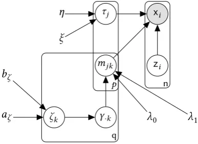
ζ_k |a_ζ,b_ζ ∼U(0,1). Furthermore, note that a_kζ encourages increasingly sparse solutions in subsequent factors. That is, related to our earlier discussion of non-identifiability (Sec-tion 2.2), we encourage loadings where the first factors have larger importance, leading to solutions that are sparse both in the rank ofMand its non-zero entries. Figure 6 presents a DAG of the spike-and-slab prior

xi

zi

τ_j

m_jk

γ·k

ζ_k a_ζ

b_ζ

n

q

λ₀ λ₁

η

ξ

p

Figure 6.Directed acyclic graph (DAG) for Bayesian factor analysis with batch effect correction for Spike-and-slab prior on the loadings matrix.

2.5

Normal-spike-and-slab

2.5.1 Formulation

We first describe the Normal-spike-and-slab prior by George and McCulloch (1993) were the spike is a Normal density with a small varianceλ₀and the slab a Normal distri-bution with large varianceλ₁. The Normal-spike-and-slab is

p(m_jk |γ_jk =l,λ_l)=N(m_jk; 0,λ_l), (2.21) withl ={0,1}. The continuity of the spike distribution gives closed form expressions for the EM algorithm, making it computationally appealing. We refer to (2.21) as Normal-SS.

2.5.2 EM algorithm for Normal-SS

Akin to the Flat prior, we outline an EM algorithm to infer∆=(M,T,ζ). Algorithm 2 summarises this maximisation.

re-Algorithm 2:EM algorithm for factor analysis model with spike-and-slab p(M)

initialiseMb=M

(0)_,

b

T =T(0),ζb=ζ

(0)

whileε >ε∗,ε_M >ε_M∗ andt <T do E-step:

Latent factors: E[zi|b∆,X]=(Iq +Mb

>

b TMb)

−1 b

M>

b Tx_i Latent indicators+: E[γjk |b∆]=pbjk

M-step:

Loadings+: mbjk =arg maxm_jkQ1(b∆) Precision: Tb

−1₌ 1

n+η−2diag

n Í

i

xix>i −2xiE[zi |b∆,X]

>

b M>

+MbE[zizi>|b∆,X]Mb

>

+ηξIp

o

Weights: ζbk =

Íp

j=1pbjk+

aζ

k −1

aζ

k +bζ+p−1

set∆(t+1)=b∆andM

(t+1)₌

b

M

computeε=Q(∆t+1) −Q(∆t),ε_M =max||m(_jkt+1)−m_jk(t)||andt =t+1

end

+_{see Sections 2.5.2, 2.6.2, 2.8.2 and 2.9.2 for details.}

spect to the latent variables and conditioning upon the currentb∆:

Q(∆) ∝_Ez,γ|

b∆,X[logp(X,Z,γ |M,T,ζ)+logp(M,T,ζ)] (2.22) Due to the conjugate Normal-SS hierarchical construction, Expression (2.22) can be split in order to simplify the EM algorithm asQ(∆)=C+Q₁(M,T )+Q₂(ζ), where:

Q₁(M,T )=− 1

2

n

Õ

i=1 h

x>

iTxi−2x>i TME[zi | b∆,X]+tr

M>

TM_E[z_iz_i>|b∆,X] i

+n+η−2

2 log| T | −

ηξ

2 tr(T ) (2.23)

− 1

2

p

Õ

j=1

q

Õ

k=1 m2

jkE

1

(1−γ_jk)λ₀+γ_jkλ₁ |b∆

,

Q₂(ζ)= p

Õ

j=1

q

Õ

k=1

log

ζ

k

1−ζ_k

b

p_jk+

q

Õ

k=1

(aζ

k −1)log(ζk)+(p+bζ −1)log(1−ζk)

,

(2.24)

wherepbjk =E[γjk |b∆]=p(γjk =1|b∆).

Expression (2.23) resembles the one for the flat prior in Section 2.2.3, plus an extra conditional expectation:

E

1

(1−γ_jk)λ₀+γ_jkλ₁ |b∆

= 1−pbjk

λ₀ +

b

withpbjk =p(γjk =1|b∆)given by b

p_jk = p(mbjk |γjk =1,λ1)p(γjk =1)

p(m_bjk |γ_jk =0,λ₀)p(γ_jk =0)+p(m_bjk |γ_jk =1,λ₁)p(γ_jk =1)

= 1

1+

q_λ

1

λ₀exp

−1₂m_b2_jkλ1

0 −

1

λ₁

1−E[ζj] E[ζj]

. (2.25)

Equation (2.25) is analogous to the EM posterior update form_jkin a two-component Gaus-sian mixture (Roˇckov´a and George, 2014).

The first and second momentsE[zi | b∆,X]andE[ziz

>

i | b∆,X]respectively are given in Equations (2.13) and (2.14) respectively.

The M-step. We proceed by optimisingQ₁andQ₂independently, in 2 steps: a

max-imisation ofQ₁with respect toM andT, followed by a maximisation ofQ₂with respect toζ. Setting to 0 the partial derivatives with respect toM gives:

∂Q

∂M =−

1 2

n

Õ

i=1 h

−2TbxiE[z

>

i |b∆,X]+2TbMbE[ziz

>

i |b∆,X] i

−Mb◦E[Dγ |b∆]=0, (2.26) withD_γ ∈’p×q,d_jk = _(1−γ 1

jk)λ0+γjkλ1 andA◦Bbeing the Hadamard (element-wise)

prod-uct of two matricesAandB. Taking thejth row of matrixM and solving equation (2.26) we obtain:

b

m_j =

" n Õ

i=1

b

τ_jx_ijE[z>i | b∆,X]

# "

diag{_E[d_j1| b∆], . . . ,E[djq |b∆]}+

n

Õ

i=1

bτjE[ziz

>

i |b∆,X]

#−1

,

(2.27) forj =1, . . . ,p.

The partial derivative w.r.t.T is the same as Equation (2.17). However the new update for the loadingsMbleads to a different solution, namely

b

T−1= 1

n+η−2diag

( _n Õ

i=1

xix>i −2xiE[zi |b∆,X]

>

b

M>₊

b

M_E[z_iz_i>|b∆,X]Mb

>_+ηξ

I_p

)

.

(2.28)

Finally,

∂Q₂ ∂ζ_k =

Íp

j=1bpjk

b

ζ_k −ζb_k2

+

aζ

k −1

b

ζ_k −

p+b_ζ −1 1−bζ_k

Solving Equation (2.29):

b

ζ_k =

Íp

j=1bpjk+

a_ζ k −1 a_ζ

k +bζ +p−1

. (2.30)

2.6

Laplace-spike-and-slab

2.6.1 Formulation

The Normal-SS prior does not give exact zeroes for the loadingsMb. We now formu-late the Laplace-spike-and-slab, (Laplace-SS). Laplace-SS was introduced by Roˇckov´a and George (2018) and is a two-component mixture of double exponentials that shrinks small values of the loadings to exact zeroes. Its heavy tails and continuity make them appealing for FA, providing closed-form updates for the EM algorithm. Laplace-SS is of the form

p(m_jk |γ_jk,λ₀,λ₁)=(1−γ_jk)Laplace(m_jk; 0,λ₀)+γ_jkLaplace(m_jk; 0,λ₁), (2.31) with a slab component with variance2λ2₀, and a spike component with2λ2₁, where

Laplace(m_jk; 0,λ)= 1

2λexp

_{− |}m

jk |

λ

.

2.6.2 EM algorithm for Laplace-SS

The E-stepThe expected complete-data log-posterior is the sum of two components.

The first component is

Q₁(M,T )=− 1

2

n

Õ

i=1 h

x>

i Txi−2x>i TME[zi |b∆,X]+tr

M>

TM_E[z_iz>_i | b∆,X] i

+n+η−2

2 log|T | −

ηξ

2 tr(T ) −

p

Õ

j=1

q

Õ

k=1

|m_jk|_{E 1−}γ

jk

λ₀ + γ_jk

λ₁ |b∆

.

(2.32)

andQ₂has the same form as (2.24). For (2.32) we set

E

₁₋γ

jk

λ₀ + γ_jk

λ₁ | b∆

= 1−bpjk

λ₀ +

b

p_jk λ₁,

withE[zi | b∆,X]andE[ziz

>

The conditional expectation forQ₂,E[γjk |b∆]=p[γjk =1|mjk]=pbjkis b

p_jk = p(mbjk |γjk =1,λ1)p(γjk =1)

p(m_bjk |γ_jk =0,λ₀)p(γ_jk =0)+p(m_bjk |γ_jk =1,λ₁)p(γ_jk =1)

= 1

1+ λ1

λ₀ exp

−|m_bjk|

1

λ₀ − λ1₁

1−_E[ζ_j]

E[ζj]

(2.33)

The M-stepupdate forMis obtained by setting to 0 the partial derivatives which are

defined form_jk ,0, and considering separately the non-differentiability pointsmjk =0. Form_jk ,0we have

∂Q

∂M =−

1 2

n

Õ

i=1 h

−2Tx_iE[z>_i |∆b,X]+2TME[ziz

>

i |b∆,X] i

−Dγ,M =0, (2.34)

withDγ,M ∈ ’p×q with element(j,k)being: dγ_jk,M = sign(m_jk)_E[d_jk | b∆]. To maximise (2.32), we consider a coordinate descent algorithm (CDA) that leads to closed-form up-dates. Viewing (2.34) with respect tom_jk, whenm_jk ,0we obtain:

∂Q₁ ∂m_jk =−

n

Õ

i=1

bτj jE[zikz

>

ik | b∆,X] !

b

m_jk+

n

Õ

i=1 "

b

τ_{j j}x_ijE[zik |b∆,X]

− q

Õ

r,k b

m_jrbτj jE[zirz

>

ik | b∆,X] #

−sign(m_bjk) "

1−p_bjk

λ₀ +

b

p_jk λ₁

# !

=ambjk+b+c ·sign(mbjk)=0

(2.35)

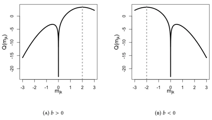
for j = 1, . . . ,p, where(a,b,c)do not depende onm_jk and are given in the first line of Equation (2.35). The solution to (2.35) is then compared tom_jk. Lemma 2.1 summarises the global maximum for the loadings.

Lemma 2.1. Letf(m_jk)= a₂m2_jk+bm_jk+c|m_jk|, wherea<0andc < 0. Definem+_jk = −(b_a+c) andm−_jk = −(b_a−c).

Ifb > −c, thenm_jk+ = arg max_mjk f(m_jk). Ifb < c, thenm−_jk = arg max_mjk f(m_jk). If

c ≤b ≤ −c, then0=arg max_mjk f(m_jk).

Proof. Our purpose is to find the maximum of f(m_jk) = a₂m2_jk +bm_jk +c|m_jk|, where

a<0, andc <0. Setting ∂Q1

∂mjk =0, we obtain

∂Q₁

∂m_jk =amjk+b+c·sign(mjk)=0.

Thus

arд max

mjk≥0f(mjk)=    

  

m+_jk := −(b_a+c) b >−c

0 otherwise

• Form_jk <0, we look for the solutions ofam_jk+b−c =0. Thus

arд max

m_jk≤0f(mjk)=    

  

m−

jk := −(ba−c) b <c

0 otherwise

Figure 7 presents a visual representation ofQ₁in function ofm_jkfor different values of

b. The updates forTb andζbk are the ones given in Equations (2.28) and (2.30) respectively.

(a)b>−c (b)c<b <−c (c)b<c

Figure 7.Maximisation ofm_jkfor Laplace-SS.

A potential concern with Normal-SS and Laplace-SS is that the slab density assigns non-negligible probability to regions of the parameter space that are also consistent with the spike, namely whenm_jk lies close to zero. We will address this via non-local priors and show that these, by enforcing separation between the two components, help increase sensitivity.

2.7

Non-local priors

Definition 2.2. An absolutely continuous measure with density p(m_jk|γ_jk =1)is a non-local prior iflim_mjk→0p(mjk|γjk =1)=0.

We call any prior not satisfying Definition 2.2 a local prior. Non-local priors possess ap-pealing properties for Bayesian model selection. They discard spurious parameters faster as the sample sizengrows, but preserve exponential rates to detect important coefficients (Johnson and Rossell, 2010) and can lead to improved parameter estimation shrinkage (Rossell and Telesca, 2017). To illustrate the motivation for NLPs in our setting consider Figure 8. Normal-SS assigns positive probability tom_jk = 0. Correspondingly, the

condi-tional inclusion probability p(γ_jk = 1 | m_jk)remains non-negligible, even whenm_jk = 0

(lower left panel).

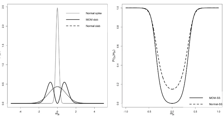
2.8

Normal-spike-and-MOM-slab

2.8.1 Formulation

Figure 8.Prior comparison (left panel) formjkunder Normal-SS and

MOM-SS and its inclusion probabilities p(γ_jk |m_jk)(right panels). Scales (λ₀,λ1) are

set to the defaults from Section 2.10.

As an alternative to the Normal-SS, we consider a product moment (pMOM) prior (Johnson and Rossell, 2012).

p(m_jk |γ_jk =0,λe₀)=N(m_jk; 0,eλ₀), p(m_jk |γ_jk =1,λe₁)=

m2

jk

e

λ₁ N(mjk; 0,eλ1).

We refer to (2.36) as MOM-SS. This prior assigns zero density tom_jk = 0givenγjk = 1, which implies p(γ_jk = 1 | m_jk = 0) = 0(Figure 8). Prior elicitation foreλ₀andeλ₁is dis-cussed in Section 2.10. From a computational point of view, the EM algorithm can accom-modate this extension by using a trivial extra gradient evaluation at negligible additional cost relative to the Normal-SS. Parameter estimation and algebraic details are described in Section 2.8.2. The prior on the inclusion indicators is set as in Equation (2.20).

2.8.2 EM algorithm for MOM-SS

The E-step: Analogous to Local spike-and-slabs (L-SSs), we first take the expected

complete-data log-posteriorQ(∆)=C+Q₁(θ,M,β,T_bi)+Q₂(ζ). By constructionQ₂is of the same form than in Equation (2.24) andQ₁is given by

Q₁(θ,M,β,T )=− 1

2

n

Õ

i=1 h

x>

iTxi−2x>iTME[zi | b∆,X]+tr

M>

TM_E[z_iz_i>|b∆,X] i

+n+η−2

2 log| T | −

ηξ

2 tr(T )

− 1

2

p

Õ

j=1

q

Õ

k=1 m2

jkE

h

d_jk |b∆ i

+

p

Õ

j=1

q

Õ

k=1

E[γjk | b∆]log(m2_jk).

(2.37)

E[zi|b∆,X]andE[ziz

>

i | b∆,X] are the same as in Equations (2.13) and (2.14) respec-tively for the Flat priors. The new conditional expectation for the inclusion probability

E[γjk |b∆]=pbjk is

b

p_jk = 1

1+ eλ₁ e m2 jk r e λ₁ e λ₀exp

−1₂m_b2_jk1 e λ₀ −

1

e λ₁

1−E[ζj] E[ζj]

(2.38)

andE[djk | b∆]=E

1 (1−γ_jk)eλ₀+γ_jkeλ₁

|b∆

= 1−bpjk e λ₀ +

b p_jk

e λ₁.

The M-step: We use a coordinate descent algorithm (CDA) that performs

succes-sive univariate optimisation on (2.37) with respect to eachm_jk, in order to maximise the loadings. An advantage is that the updates have a closed-form that is computationally inexpensive. As a potential drawback it could require a larger number of iterations to converge relative to performing joint optimisation with respect to multiple elements in