warwick.ac.uk/lib-publications Manuscript version: Author’s Accepted Manuscript
The version presented in WRAP is the author’s accepted manuscript and may differ from the published version or Version of Record.
Persistent WRAP URL:
http://wrap.warwick.ac.uk/116855
How to cite:
Please refer to published version for the most recent bibliographic citation information. If a published version is known of, the repository item page linked to above, will contain details on accessing it.
Copyright and reuse:
The Warwick Research Archive Portal (WRAP) makes this work by researchers of the University of Warwick available open access under the following conditions.
Copyright © and all moral rights to the version of the paper presented here belong to the individual author(s) and/or other copyright owners. To the extent reasonable and
practicable the material made available in WRAP has been checked for eligibility before being made available.
Copies of full items can be used for personal research or study, educational, or not-for-profit purposes without prior permission or charge. Provided that the authors, title and full
bibliographic details are credited, a hyperlink and/or URL is given for the original metadata page and the content is not changed in any way.
Publisher’s statement:
Please refer to the repository item page, publisher’s statement section, for further information.
A Numerical Study on the
Hydrodynamics of Standing Waves in
front of Caisson Breakwaters by a
WCSPH Model
Yeganeh-Bakhtiary, A, Houshangi, H, Hajivalie, F & Abolfathi, S
Original citation & hyperlink:
Yeganeh-Bakhtiary, A, Houshangi, H, Hajivalie, F & Abolfathi, S 2016, 'A Numerical Study on the Hydrodynamics of Standing Waves in front of Caisson Breakwaters by a WCSPH Model' Coastal Engineering Journal, vol 59, no. 2, 1750005
https://dx.doi.org/10.1142/S057856341750005X
DOI 10.1142/S057856341750005X ISSN 0578-5634
ESSN 1793-6292
Publisher: World Scientific Publishing
Electronic version of an article published as [Coastal Engineering Journal, 59, 1, 2016, 1750005] [10.1142/S057856341750005X] © copyright World Scientific Publishing Company http://www.worldscientific.com/worldscinet/cej
Copyright © and Moral Rights are retained by the author(s) and/ or other copyright owners. A copy can be downloaded for personal non-commercial research or study, without prior permission or charge. This item cannot be reproduced or quoted extensively from without first obtaining permission in writing from the copyright holder(s). The content must not be changed in any way or sold commercially in any format or medium without the formal permission of the copyright holders.
1
A Numerical Study on Hydrodynamics of Standing Waves in front of Caisson
Breakwaters with WCSPH Model
Abbas Yeganeh-Bakhtiary1,2, Hamid Houshangi3, Fatemeh Hajivalie4 and Soroush Abolfathi5
1
School of Civil Engineering, Iran University of Science & Technology, Narmak, Tehran 16844, Iran,
2
Civil Engineering Program, Faculty of Engineering, Universiti Teknologi Brunei (UTB), Gadong
BE1410, Brunei Darussalam, [email protected]
3
PhD candidate, School of Civil Engineering, IUST, Narmak, Tehran 16844, Iran, [email protected]
4
Iranian National Institute for Oceanography & Atmospheric Sciences, Tehran, 1411813389, Iran,
Coventry CV15FB, UK, Coventry University,
, Flow Measurement & Fluid Mechanics Research Center
5
2
Abstract
In this paper a two-dimensional Lagrangian model based on the weakly compressible smoothed particle hydrodynamics (WCSPH) was developed to explore the hydrodynamics of standing waves impinge on a caisson breakwater. The developed model is validated against experimental data and applied then to analyze the wave horizontal velocity in front of a vertical caisson. The effect of wall steepness was investigated in terms of the steady streaming pattern due to generation of fully to partially standing waves. The numerical results indicated that the partially standing waves generated in front of the sloped caisson change the pattern of steady streaming. For the vertical caisson, the velocity component of recirculating cells increased in front of the vertical wall; whereas, for the sloped caisson it decreased from the sloped wall with reducing the wall steepness. In addition, near the milder sloped wall the intensity of velocity component is higher, which is an important parameter in scour process in front of caisson breakwater.
3
1. Introduction
4
surface becomes very difficult. To overcome these difficulties, using the mesh-free particle methods might be a superior approach.
The particle methods solve the N-S equations with complicated boundary conditions by using a set of discrete particles based on Lagrangian formalism. Additionally, Lagrangian behavior of particles, resolves the problem associated with grid-based calculations by computing the convection terms without the numerical diffusion [Liu and Liu, 2003; Khayyer et al., 2008]. Among the particle methods, the Smoothed Particle Hydrodynamics (SPH) is widely employed to simulate the incompressible fluid flows. Generally, there are two discernible approaches of SPH available for modeling the incompressible flows; namely weakly compressible SPH (WCSPH), and incompressible SPH (ISPH). The main difference between the two approaches is how to estimate the pressure filed. In the former approach, a state equation is implemented [e.g., Colagrossi and Landrini, 2003; Dalrymple and Rogers, 2006; Becker and Teschner, 2007; Altomare et al., 2015]; whilst, in the latter one the Poisson equation is solved for the pressure estimation [e.g. Cummins et al., 1999; Shao, 2006; Shao and Lo, 2003; Gotoh et al., 2014; Gotoh and Khayyer, 2016].
5
performance and the flexibility of WCSPH are successfully tested in coastal engineering problems [Monaghan and Kos, 1999; Kim and Ko, 2008; Mahmoudi et al., 2014; Altomare et al., 2015; Liu and Liu, 2016]. In this study, the WCSPH was adopted for two folds: (i) the WCSPH is rather easier to program; and (ii) the pressure calculation and volume conservation can be easily achieved for standing waves in front of a caisson breakwater.
On the other hand, a substantial knowledge has been accumulated so far on the steady streaming under the fully standing waves; however, very little is known about the hydrodynamics of the partially standing waves in front of caisson breakwaters. The main purpose of the present work is to numerically study the wall steepness effects on the hydrodynamics of partially standing waves via the applicability of WCSPH model. The model was developed to simulate the hydrodynamic process during interactions of standing waves with vertical and sloped caisson breakwaters. The numerical result was first validated using both the experimental data and analytical solution. Then it is applied to the vertical caisson with different wave properties based on Xie [1981] and Zhang et al. [2001] experiments to systematically analyze the orbital horizontal velocity. Finally, the developed WCSPH model was implemented to study the hydrodynamics of partially standing waves in front of caisson breakwaters with different slopes to investigate the wall steepness effects on the pattern of steady streaming.
2. Mathematical Formulation
2.1. Governing equations
6
1
𝜌 𝑑𝜌
𝑑𝑑+∇.𝑢�⃗ = 0 (1)
𝑑𝑢�⃗ 𝑑𝑑 =−
1
𝜌 ∇𝑃+
1
𝜌 ∇(𝜇.∇𝑢�⃗) +
1
𝜌 ∇.𝜏+𝑔⃗ (2)
where 𝑢�⃗ is flow velocity vector, 𝑃 and𝜌 are respectively pressure and density, t is time marching,
𝑔⃗= (0,0,−9.81) 𝑚/𝑠2 is the gravitational acceleration,∇ is the vector differential operator, µ is
the kinematic viscosity, and 𝜏 is the SPS stress tensor. Eq. 1 is in the form of a compressible flow; while in the momentum equation, Eq. 2, the effect of viscosity is very important. The viscous effect can be simulated by the artificial viscosity [Monaghan, 1992] or by the approximated laminar viscosity [Morris et al., 1997]. Excluding the artificial viscosity and the laminar viscosity, the Sub-Particle Scale (SPS) approach was adopted in this study. The SPS approach was initially introduced by Gotoh et al. [2001] in the context of Moving Particle Semi-implicit method (MPS); hence, to apply it for a compressible fluid, a special averaging method is required. In the current study, the so-called Favre-averaging scheme was adopted, which is a density-weighted time averaging approach [Dalrymple and Rogers, 2006].
Using the Favre-averaging scheme for compressible fluid flow, the eddy viscosity assumption based on the Boussinesq's hypothesis is often used to model the SPS stress tensor (𝜏𝑖𝑖) as
𝜏𝑖𝑖 =𝜌 �2𝜈𝑡𝑆𝑖𝑖−23𝑘𝑆𝑆𝑆𝛿𝑖𝑖� −23𝜌𝐶𝐼Δ2𝛿𝑖𝑖�𝑆𝑖𝑖�2 (3)
where 𝐶𝐼 is a constant that set to 0.0066 according to Blinn et al. [2002], 𝑘𝑆𝑆𝑆 is the SPS turbulence kinetic energy, ∆is the initial particle-particle spacing, 𝑆𝑖𝑖 is the element of SPS strain-rate tensor, 𝜈𝑡 is the turbulent eddy viscosity, and 𝛿𝑖𝑖 is Kronecker delta.
7
𝜈𝑡 = (CsΔ)2. |𝑆| (4)
here 𝐶𝑠 = 0.12 is the Smagorinsky constant and |𝑆| =�2𝑆𝑖𝑖𝑆𝑖𝑖�1 2⁄ is the local strain rate.
2.2. SPH formulation
To get a particular quantity at an arbitrary point 𝑥 of the fluid domain, SPH uses the following interpolation
𝑓(𝑥) =� 𝑓𝑏𝑊(𝑥 − 𝑥𝑏)𝑚𝜌𝑏 𝑏 𝑏
(5)
where 𝑓𝑏 is the value of function 𝑓associated with particle 𝑏 located at 𝑥𝑏, 𝑊(𝑥 − 𝑥𝑏) is the weighting function determining the contribution of particle 𝑏 to the value of 𝑓 at 𝑥, and 𝑚𝑏 and𝜌𝑏 are the mass and density of particle 𝑏, respectively. The variable of 𝑊(𝑥 − 𝑥𝑏) is usually called the kernel function and its amount varies from 0 to 1. By considering the computational accuracy, a cubic spline function was adopted among various kinds of kernel functions known as the B-spline function and specified by [Monaghan, 1992]:
⎩ ⎪ ⎨ ⎪
⎧ 𝑊(𝑟,ℎ) =710𝜋ℎ2�1−32𝑞2+3
4𝑞3� 𝑞< 1
𝑊(𝑟,ℎ) =2810𝜋ℎ2(2− 𝑞)3 1 <𝑞 < 2 𝑊(𝑟,ℎ) = 0 𝑞 > 2
(6)
8
summation to include only the neighboring particle of the particle𝑎. This technique leads to a great saving in both of the time and calculation effort.
On the basis of the above discussion, the N-S equations are closured with the SPS turbulence model to simulate the flow motion, described in the SPH notation as follows:
�𝑑𝜌𝑑𝑑�
𝑎 =� 𝑚𝑏 𝑏𝑢�⃗𝑎𝑏.∇𝑊𝑎𝑏 (7)
�𝑑𝑢�⃗𝑑𝑑 � 𝑎
=− � 𝑚𝑏�𝜌𝑃𝑎 𝑎2+
𝑃𝑏
𝜌𝑏2� ∇𝑊𝑎𝑏+�
4𝑚𝑏𝜇𝑟⃗𝑎𝑏.∇𝑊𝑎𝑏
(𝜌𝑎+𝜌𝑏)(𝑟𝑎𝑏2 +𝜙2) 𝑏
𝑏
𝑢�⃗𝑎𝑏
+� 𝑚𝑏�𝜌𝜏𝑎 𝑎2+
𝜏𝑏
𝜌𝑏2� ∇𝑊𝑎𝑏+𝑔⃗ 𝑏
(8)
where 𝑎 and 𝑏 denote respectively the reference particle and its neighbors, 𝑢�⃗𝑎𝑏=𝑢�⃗𝑎− 𝑢�⃗𝑏,
𝑟⃗𝑎𝑏=𝑟⃗𝑎− 𝑟⃗𝑏, and 𝜙is a small number introduced to keep the denominator non-zero and usually
is 0.1ℎ𝑎𝑏.
Incompressibility approximation is a common trick in the SPH formulation, hence, in this model the incompressible flow condition was assumed with a weak compressibility. In other words, instead of solving the Poisson equation to approximate the pressure field, a state equation is utilised. In the state equation, the sound speed, set to at least ten times of the maximum fluid velocity, is used for the calculation of coefficients. To satisfy the Courant–Friedrichs–Lewy (CFL) condition, the time step is limited to a very small value that slows down the simulation efficiency [Monaghan, 1992]. Compressibility causes problems with the sound wave reflection at the boundaries; due to its simplicity, however, the state equation is still widely used in the pressure calculation of the simulations. The state equation is
𝑃 =𝐵 ��𝜌𝜌 0�
𝛾
9
here 𝛾 = 7 is a constant, 𝐵 =𝑐02𝜌0⁄𝛾 in which the 𝜌0 is the reference density, 𝑐0 is the speed of sound at the reference density, and 𝑐0 = 𝑐(𝜌0) =�∂𝑃 𝜕𝜌⁄ . The exact sound speed was not used because it requires very small time steps to ensure the numerical stability [Monaghan, 1992]. The appropriate sound speed was chosen large enough to keep the relative density fluctuation small [Monaghan, 2005]. In fact, the advantage of implementing this technique is to define a direct relation between the flow pressure and the fluid’s local density; consequently, there is no need to solve the Poisson equation to approximate the fluid pressure.
2.3 Particles movement and time marching
Particles in the numerical domain move according to the following equation:
�𝑑𝑟⃗
𝑑𝑑�𝑎 =𝑢�⃗𝑎+𝜀 � 𝑚𝑏 𝜌̅𝑎𝑏 𝑏
(𝑢�⃗𝑏− 𝑢�⃗𝑎)𝑊𝑎𝑏 (10)
here 𝜀 is a constant (= 0.5) and 𝜌̅𝑎𝑏= (𝜌𝑎+𝜌𝑏) 2⁄ . The last term in the equation is called XSPH correction, which guarantees that the neighboring particles possess approximately the same velocity components [Monaghan, 1994].
In this study, an Euler Predictor-Corrector time marching scheme was employed to develop the solution of the WCSPH equations with time [Monaghan, 1989]. Considering respectively the momentum (Eq. 2), density (Eq. 7) and position (Eq. 10) equations, in the following form
⎩ ⎪ ⎨ ⎪ ⎧𝑑𝑢�⃗𝑎
𝑑𝑑 = 𝐹⃗𝑎 𝑑𝜌𝑎
𝑑𝑑 =𝐷𝑎 𝑑𝑟⃗𝑎
𝑑𝑑 =𝑈��⃗𝑎
10
where 𝑈��⃗𝑎 represents the velocity contribution of particle 𝑎 from the neighboring particles (XSPH correction). This scheme predicts the time-marching progress as
⎩ ⎪ ⎨ ⎪
⎧𝑢�⃗𝑎𝑛+1/2 = 𝑢�⃗𝑎𝑛 +∆𝑑2 𝐹⃗𝑎𝑛
𝜌𝑎𝑛+1/2 = 𝜌𝑎𝑛 +∆𝑑2 𝐷𝑎𝑛
𝑟⃗𝑎𝑛+1/2 = 𝑟⃗𝑎𝑛 +∆𝑑2 𝑈��⃗𝑎𝑛
(12)
computing 𝑃𝑎𝑛+1/2 =𝑓(𝑃𝑎𝑛+1/2) with Eq. 9. The updated value of the above-mentioned variables are then corrected using forces at the half time step
⎩ ⎪ ⎨ ⎪
⎧𝑢�⃗𝑎𝑛+1/2 = 𝑢�⃗𝑎𝑛 +∆𝑑2 𝐹⃗𝑎𝑛+1/2
𝜌𝑎𝑛+1/2 = 𝜌𝑎𝑛 +∆𝑑2 𝐷𝑎𝑛+1/2
𝑟⃗𝑎𝑛+1/2 = 𝑟⃗𝑎𝑛 +∆𝑑2 𝑈��⃗𝑎𝑛+1/2
(13)
Finally, the values are calculated at the end of the time step following:
�
𝑢�⃗𝑎𝑛+1= 2𝑢�⃗𝑎𝑛+1/2− 𝑢�⃗𝑎𝑛 𝜌𝑎𝑛+1 = 2𝜌𝑎𝑛+1/2− 𝜌𝑎𝑛 𝑟⃗𝑎𝑛+1 = 2𝑟⃗𝑎𝑛+1/2− 𝑟⃗𝑎𝑛
(14)
The pressure was calculated from the density using both 𝑃𝑎𝑛+1/2 =𝑓(𝑃𝑎𝑛+1/2) and Eq. 9.
Practically, the midpoint values of the previous time step were used instead of computing the values at time𝑛; it saves computational time and produces only a negligible error. The afore-mentioned scheme is second order and conserves both the linear and angular momentum [Monaghan, 1989].
11
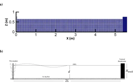
A rectangular computational domain was considered in this study (Fig. 2). The spatial discretization of computational domain was set up with the initial arrangement of particles. At the inlet boundary, a hinged flap wavemaker was considered and at the outlet and bottom boundaries, solid walls were used to prevent the inner particles from penetrating into the boundaries. In the present study, the treatment of wall boundaries was simulated similar to the model of Koshizuka et al. [1998]. In order to keep the density at the wall in consistent with that of the inner particles, several lines of dummy particles were placed outside the solid wall. The velocity of boundary particles were set to zero to satisfy no-slip boundary condition; while, to obtain the pressure for dummy particles the homogeneous Neumann conditions were applied. The lack of enough particles near or on the boundary is an important issue in SPH, resulting from truncation of the integral in the boundary region. For particles near or on the boundary, only particles inside the boundary contribute to the summation of the particle interface, and no contribution comes from the outside since there are no particles beyond the boundary. With a basic discretization, it was observed that particles can penetrate and even cross the walls; as a result, a repulsive force and ghost particles were employed here.
12
increased due to the pressure term, 𝑃𝑎⁄𝜌𝑎2, in the momentum equation, and therefore that particle cannot penetrate into the boundary.
As stated before, the fluid particles were initially arranged in a regular form. The initial computational domain of the problem was discretized with separate particles [see Fig. 2]. In the computation process a constant time step of ∆𝑑= 4.5 × 10⁻⁵ s was employed and the time duration of simulation was equal to ten wave period time for each case study.
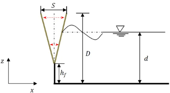
A flap type wavemaker was utilized to generate the wave in the numerical domain. The schematic sketch of the wavemaker is depicted in Fig. 3. The Stokes wave theory was applied to generate the incident wave at the inlet boundary; to generate the Stokes wave by the flap type wavemaker, the relation between the flap stroke length (𝑆), water depth (𝑑) and wave height (𝐻) is given according to Dean and Dalrymple [1984] as
𝑆=H2(coshsinh𝑘𝑑𝑘𝑑 −+𝑘𝑑1) (15)
then the displacement of the flap is given by
𝑥𝑓(𝑑) =12�(𝑧 − ℎ𝑓)/(𝐷 − ℎ𝑓)�×𝑆× sin (𝜔𝑑) (16)
where 𝑥𝑓 is the displacement of flap particles at corresponding 𝑧 location, ℎ𝑓 and 𝐷 are the beginning and the end of flap in 𝑧 direction, respectively. Here ℎ𝑓 is set to zero (ℎ𝑓 = 0).
3. Result and Discussions
3.1. Model validation
13
experimental configurations was 0.75 m. The standing waves were generated in still water depths of 0.55, 0.60, and 0.65 m; with the incident wave heights of 0.09, 0.12, 0.15, and 0.18 m. For the wave heights greater than 0.09 m the wave overtopping occurs. In the experiments the wave steepness (H/L) ranged from 0.021 to 0.068 and the relative water depth (d/L) ranged from 0.139 to 0.353. The horizontal particle velocity was measured at 0.25 m from the bed near the first node of standing waves. In the numerical simulations, the cases with no overtopping considered, in which the incident wave height set to 0.09 m. Table 1 summarizes the specifications of three test cases of Lagrangian model based on Zhang et al. [2001] experiment.
Xie [1981] experiments carried out in a wave flume with 38 m long, 0.8 m wide and 0.6 m deep. The water depth is equal to 0.45 m in the beginning of the flume and reaches to 0.3 m at the flat bed near the breakwater by a 1:30 slope. Fig. 4 depicts schematically the sketch of Xie [1981] experimental set up. He measured the distribution of the horizontal velocity of water particles in front of a caisson breakwater at nodes and between nodes and antinodes and compared the experimental results with those of the linear wave theory and Miche [1944] second order standing wave theory. In the experiments, wave steepness,𝐻/𝐿, ranged from 0.0083 to 0.0375, relative water depths 𝐻/𝑑ranged from 0.05 to 0.175 (where 𝐻and𝐿 are respectively the incident wave height and length, and 𝑑is the water depth). Four test cases of numerical model properties based on Xie [1981] experiments were simulated, which characteristics are summarized in Table 2.
14
of standing wave in front of caisson breakwaters. To save the computation CPU time, the length of computational domain was reduced to 2𝐿.
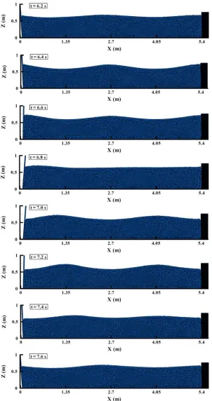
Fig. 5 shows the snapshots of standing wave generated in front of a vertical caisson in one wave period (for test No. 2). The time interval between each frame is 0.2 s after the standing wave was fully developed (𝑇= 1.4 𝑠). The figure shows the interaction of the incident and reflected waves as well as the development of standing waves and their subsequent impact on the caisson. As expected the standing wave forms the higher and more symmetric wave envelopes, during which the crest height of the standing wave reaches to twice of the crest height of incident wave in vicinity of the vertical caisson.
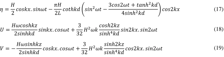
Tracking of the wave surface was performed using the Lagrangian model for two different time spot of simulation, namely at the half-wave period (𝑑 =𝑇/2) and at one-wave period (𝑑 =𝑇). Fig. 6 shows the comparison of wave configuration between the numerical result and the theoretical wave solution for test No. 2. The finite-amplitude standing waves based on Miche [1944] theory was adopted, in which the water elevation profile 𝜂 and velocities components
𝑈and 𝑉are expressed as follows:
𝜂 =𝐻2𝑐𝑐𝑠𝑘𝑥.𝑠𝑠𝑛𝜔𝑑 −𝜋𝐻2𝐿 𝑐𝑐𝑑ℎ𝑘𝑑 �𝑠𝑠𝑛2𝜔𝑑 −3𝑐𝑐𝑠2𝜔𝑑+𝑑𝑎𝑛ℎ2𝑘𝑑
4𝑠𝑠𝑛ℎ2𝑘𝑑 � 𝑐𝑐𝑠2𝑘𝑥 (17)
𝑈 =𝐻𝜔𝑐𝑐𝑠ℎ𝑘𝑧
2𝑠𝑠𝑛ℎ𝑘𝑑 𝑠𝑠𝑛𝑘𝑥.𝑐𝑐𝑠𝜔𝑑+
3
32𝐻2𝜔𝑘
𝑐𝑐𝑠ℎ2𝑘𝑧
𝑠𝑠𝑛ℎ4𝑘𝑑 𝑠𝑠𝑛2𝑘𝑥.𝑠𝑠𝑛2𝜔𝑑 (18) 𝑉 =−𝐻𝜔𝑠𝑠𝑛ℎ𝑘𝑧2𝑠𝑠𝑛ℎ𝑘𝑑 𝑐𝑐𝑠𝑘𝑥.𝑐𝑐𝑠𝜔𝑑+323 𝐻2𝜔𝑘𝑠𝑠𝑛ℎ2𝑘𝑧
𝑠𝑠𝑛ℎ4𝑘𝑑 𝑐𝑐𝑠2𝑘𝑥.𝑠𝑠𝑛2𝜔𝑑 (19)
[image:16.612.72.541.486.606.2]15 𝐿=2𝑔𝜋 𝑇2𝑑𝑎𝑛ℎ2𝜋𝑑
𝐿 (20)
As seen from Fig. 6, the numerical results match well with the predication of finite amplitude wave; however, a slight difference between the numerical result and the theoretical value was observed. This difference is due to the Lagrangian behavior of the WCSPH model.
To check the numerical convergence, the fluctuation of wave profile and the horizontal orbital velocity due to development of standing waves were monitored. Fig. 7 shows the time variation of water level at 𝐿/4 and 𝐿/2 from the caisson wall (see Fig. 7a and b). The free surface deformation was measured at the first antinode (𝑥= 4.05 𝑚) from the caisson wall, where the fluctuation rate is very significant. The fluctuation of horizontal orbital velocity at the first antinode and node from the caisson wall are also presented in the figure. As seen, after fluctuating for few seconds - considered as the warm up time of numerical calculation- both of the water wave profile and horizontal orbital velocity are converged.
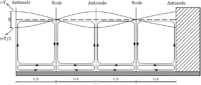
Furthermore, after fully development of standing wave, at nodes the free surface deformation is the minimum, and the maximum horizontal velocity components of fluid particle motions occur at this point; whereas the process is completely reverse at the antinodes. The same tendency was reported for the horizontal and vertical velocity components of standing waves, in front of a vertical wall [Sumer and Fredsøe, 2000]. The first node and antinode were located precisely at the position of 𝐿/4 and 𝐿/2 from of the caisson wall, respectively.
16
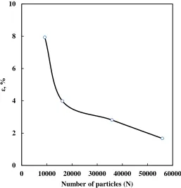
differences between the wave heights of numerically generated standing wave with that of the theoretical value by using the formulation introduced by Xu et al. [2009] as
𝜀 =��𝐻𝑛𝑛𝑛𝐻− 𝐻𝑎𝑛𝑎𝑎𝑎𝑡𝑖𝑎𝑎𝑎
𝑎𝑛𝑎𝑎𝑎𝑡𝑖𝑎𝑎𝑎 ��× 100% (21)
Fig. 8 depicts the relative error of WCSPH for different resolution ranges. The error is approximately 8% for the roughest resolution and 2% for the finest one. As seen, by increasing the number of particles, the relative error sharply decreases to reach to below 2%. For the finer resolutions, however, the error is decreasing slowly compared to the rough resolution indicating the convergence of the current WCSPH model.
To have a better insight to performance of the developed model, the pattern of steady streaming was explored sophistically in front of a caisson breakwater for test No.2. Fig. 9 plots the pattern of steady streaming generated by standing waves in front of caisson. To have a proper depiction of the figure, a non-dimensional axis in 𝑧 direction was used and denoted by𝑧/𝑑𝑑𝑑𝑑𝑎; 𝑑𝑑𝑑𝑑𝑎 =
17
shows a remarkable effect on the averaging process for the top recirculating cells in the pattern of steady streaming. The downward component of the water particle induces very high velocities at the toe of the wall and horizontally away from the wall at𝐿/4. The latter component shows its significant effect in the bottom recirculating cells.
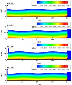
The wave pressure due to the standing wave on the vertical caisson was also estimated. The result for the evaluation of the pressure field is presented in Fig. 10. As can be seen from the figure the computed pressure fields are stable and there is no serious pressure noise, which is an indication that the pressure solution of WCSPH model is reliable. For more details, the numerical distribution of wave pressure on the vertical caisson was compared with the Sainflou empirical formula. Sainflou [1928] estimated the wave pressures induced by the standing waves on a vertical wall with assuming both the non-breaking second order wave theory and the linear pressure distribution below the water level for wave crest and trough as follows:
Wave crest:
𝑃
𝛾 =−𝑧0+𝐻 �
𝑐𝑐𝑠ℎ𝑘(ℎ+𝑧0) 𝑐𝑐𝑠ℎ𝑘ℎ −
𝑠𝑠𝑛ℎ𝑘(ℎ+𝑧0)
𝑠𝑠𝑛ℎ𝑘ℎ � (22)
at free surface (𝑧0 = 0), 𝑃 = 0; and at bottom (𝑧0 =−ℎ), 𝑃= 𝛾(ℎ+𝐻 𝑐𝑐𝑠ℎ𝑘ℎ⁄ )
Wave trough:
𝑃
𝛾 =−𝑧0− 𝐻 �
𝑐𝑐𝑠ℎ𝑘(ℎ+𝑧0) 𝑐𝑐𝑠ℎ𝑘ℎ −
𝑠𝑠𝑛ℎ𝑘(ℎ+𝑧0)
𝑠𝑠𝑛ℎ𝑘ℎ � (23)
at free surface (𝑧0 = 0), 𝑃 = 0; and at bottom (𝑧0 =−ℎ), 𝑃 =𝛾(ℎ − 𝐻 𝑐𝑐𝑠ℎ𝑘ℎ⁄ ), here 𝛾 is the water density and 𝑧0 is the origin of coordinate at water surface.
18
seen between the numerical and theoretical distribution of hydrodynamic pressure. Although the pressure fluctuation is relatively higher for the wave crest, the pressure field of standing wave in front of vertical breakwater is quite acceptable in this simulation.
Fig. 12 illustrates the distribution of the horizontal velocity of water particles for test cases No. 4 and 7. Horizontal velocities were measured in nodes and a point between nodes and antinodes at distance of 5 cm, 10 cm, and 20 cm from the bed in Xie [1981] experiments. The comparison of numerical, analytical and experimental results is shown in the figure. There are nearly good agreement between the numerical, analytical and experimental results, but there is a slight discrepancy in the numerical results compared with those of the experimental and analytical data. This discrepancy can be attributed to the Lagrangian behavior of the WCSPH model.
To study how the standing wave velocity varies with the water depth, the non-dimensional velocity is drawn against 𝑑/𝐿 in Fig. 13. In the figure, the numerical, analytical and experimental results of the non-dimensional velocity (𝑢𝑇/𝐻) are compared against the relative water depth for the test cases based on Xie [1981] experiments. In the experiment, the non-dimensional velocity (𝑢𝑇/𝐻) was measured at the first node and a point between node and antinode at 5 cm, 10 cm, and 20 cm from bed. As seen the agreement between them is acceptable; hence, it is evident that the non-dimensional velocity decreases by increasing of the relative water depth. This consequence is similar to the numerical results of the test cases based on Zhang et al. [2001] experimental data, as shown in Fig. 14.
3.3 Numerical results
19
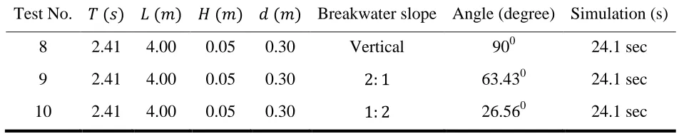
analyze the effect of the wall steepness on the pattern of standing waves, three numerical simulations were carried out. The hydrodynamic of the numerical simulations are summarized in Table 3. Three different simulations were set up in front of a vertical caisson, a 1:2 and a 2:1 sloped wall. Fig.15 gives a schematically view of the numerical domains. The simulations were performed in a numerical domain with 4 m length and 0.5 m height, water depth was equal to 0.3 m and the distant between wave generator and the caisson was 4 m, equal to a one wave length. For the case of sloped breakwater the toe of the breakwater is positioned at 𝐿′= 𝐿 − 𝑑/𝑑𝑎𝑛𝑡, where 𝑡is the angle of the sloped wall.
20
waves from a caisson wall depends on its front wall steepness. This is attributed to wave energy consumption during the rush up and rush down process [Tofany et al., 2014]. Also, Hajivalie and Yeganeh-Bakhtiary [2009] pointed out that the caisson wall steepness significantly changes not only the characteristics of the partially standing waves but also the pattern of steady streaming. To have a better understanding of the effect of wall steepness on caisson breakwaters, the standing wave configuration is illustrated in Fig. 17. The standing waves are depicted at𝑑= 𝑇/
2, and 𝑑 =𝑇 for vertical, 2:1 sloped, and 1:2 sloped caisson. As seen for the case of the fully standing waves in front of vertical caisson, the feature of maximum and minimum water free surface is rather symmetrical, but this symmetrical pattern starts to switched to the asymmetrical ones as the wall steepness increases. In addition, the positions of nodes and antinodes in 𝑥 and 𝑧 directions alter due to increase in the wall steepness. It can be seen that, the node and antinode points, in the 𝑧 direction, are descending; whereas, in the 𝑥 direction with increasing of the wall steepness these points shift towards the caisson wall. Thus, these circumstances can change the pattern of steady streaming in front of the caisson breakwaters, as well.
21
after several time steps due to Lagrangian resolution of the governing equations, however, the arrangement of fluid particles becomes very untidy. To overcome this shortcoming, a spatial averaging scheme over the whole domain of simulation was implemented with using of the kernel function in SPH.
Referring again to Fig. 18, it is noted that the orbital velocity of water particles were averaged during a whole wave period after the standing waves were completely developed. Formation of clock wise and anti-clock wise recirculating cells in front of all three breakwaters is clearly displayed in the figure. As seen, there is a slight difference in the pattern of steady streaming in front of vertical caisson with that of the steep sloped ones; in both cases the recirculating cells of steady streaming have almost regular and symmetrical pattern. In contrast, in front of the mild sloped caisson, this regularity is markedly disturbed. The velocity component of recirculating cells increased in front of the vertical caisson, but decreased away from the walls by reducing the wall steepness. Near the milder slope caisson the pattern of recirculating cells is more complicated and the intensity of velocity component increased, which is an important key in scour process at toe of the caisson wall. The pattern of recirculating cells can strongly justify the reason of occurrence of scour at toe of the sloped caisson mentioned earlier by Sumer and Fredsøe [2000].
22
vertical caisson. The figure also indicates that the difference between steep sloped and vertical breakwater is rather negligible. Fig. 19b compares the vertical distribution of horizontal mass transport velocity at a point between node and antinode near the caisson. As shown, for the milder sloped case the horizontal velocity is higher than the other cases at the lower half water depth. For three cases at the upper half of water depth the horizontal velocities are in reverse direction. It is evident that variations of the horizontal velocities of tests No. 8 and 9 are nearly the same in water column near the caisson wall.
The distribution of turbulence kinetic energy 𝑘𝑆𝑆𝑆 (𝑚2⁄𝑠2) around the 2:1 sloped caisson (test No. 10) is shown in Fig. 20. The figures present the snapshots of waves rush up and rush down over the caisson slope. As seen, the intensity of turbulent kinetic energy increases in the vicinity of free surface during the wave rush up, but the turbulent energy decreases as the wave rushes down. To have a better picture of the turbulence effect, Fig. 21 depicts the turbulent energy effect on the fluid particle movements on the sloped wall at t = T/2 (top figure) and t = T (bottom figure) for test No. 10. As seen near the milder slope caisson, the pattern of recirculating cells is rather complicated; it seems that a secondary recirculating cell is formed near the toe of caisson, which is more visible at t = T/2 (top figure). This procedure may justify the occurrence of higher scour depth near the toe of the sloped caisson, reported earlier by Sumer and Fredsøe [2000].
4. Conclusion
23
the WCSPH model to account for the turbulence effects. The hydrodynamic process induced by standing waves was explored systematically in terms of maximum horizontal velocity distribution at some key points. Also, the tracking of wave free surface and the pattern of steady streaming generated in front of caisson breakwater with different wall steepness were investigated. A wide range of experimental and analytical data was used to analyze this work. From this numerical investigation, the following conclusions are drawn:
• The numerical model provides a useful approach to improve the engineering perceptions of the kinematic and dynamic properties of the standing wave generated in front of caisson breakwaters.
• Partially standing waves, generated in front of the sloped caisson, changes the pattern of steady streaming. The velocity component of recirculating cells increased in front of the vertical caisson, but it decreased away from the walls by reducing the wall steepness, which is a key issue in scour process at toe of the caisson wall.
• The horizontal velocity of mass transport in front of vertical caisson is stronger than that of the milder sloped caisson.
• The hydrodynamic conditions in front of vertical and steep sloped caisson are nearly the same.
24
5. References
Altomare, C., Crespo, A.J.C., Domínguez, J.M., Gesteira, M.G., Suzuki, T. & Verwaest, T. [2015] “Applicability of Smoothed Particle Hydrodynamics for estimation of sea wave impact on coastal structures” Coast. Eng.96 (2), 1–12.
Becker, M. & Teschner, M. [2007] “Weakly compressible SPH for free surface flows” in Proc. of the ACM Siggraph/ Eurographics Symposium on Computer Animation, pp. 209–217. Blinn, L., Hadjadj, A. & Vervisch, L. [2002] “Large eddy simulation of turbulent flows in
reversing systems” in Proc. 1st French Seminar on Turbulence and Space Launchers. CNES, Paris.
Carter, T.G., Liu, L.F.P. & Mei, C.C. [1973] “Mass transport by waves and offshore sand bed forms” J. Waterw. Port, Coast. 99(WW2), 165-184.
Colagrossi, A. & Landrini, M. [2003] “Numerical simulation of interfacial flows by smoothed particle hydrodynamics” J. Comput. Phys. 191(2), 448–475.
Colagrossi, A., Antuono, M. & Touze, D.L. [2009] “Theoretical considerations on the free-surface role in the smoothed-particle-hydrodynamics” Phys Rev E, 79.
Cummins, S.J., Sharen, J. & Rudman, M. [1999] “An SPH projection method” J. Comput. Phys.
152(2), 584–607.
Dean, R.G. & Dalrymple, R.A. [1984] “Water Wave Mechanics for Engineers and Scientists” World Scientific publishing Company, p. 470.
25
Gislason, K., Fredsøe, J., Deigaard, R. & Sumer, B.M. [2009] “Flow under standing waves part I. Shear stress distribution, energy flux and steady streaming” Coast. Eng. 56(3), 341-362.
Gotoh, H. & Khayyer, A. [2016] “Current achievements and future perspectives for projection-based particle methods with applications in ocean engineering” J. Ocean Eng. Marine Eng.2(3), 251-278.
Gotoh, H., Khayyer, A., Ikari, H., Arikawa, T. & Shimosako, K. [2014] “On enhancement of Incompressible SPH method for simulation of violent sloshing flows” App. Ocean Res.
46, 104–115.
Gotoh, H., Okayasu, A. & Watanabe, Y. [2013] “Computational wave dynamics” World Scientific Publishing Company, p. 234.
Gotoh, H., Shibahara, T. & Sakai, T. [2001] “Sub-particle-scale turbulence model for the MPS method Lagrangian flow model for hydraulic engineering” Comp. Fluid Dyn. 9(4), 339- 347.
Hajivalie, F. & Yeganeh-Bakhtiary, A. [2009] “Numerical study of breakwater steepness effect on the hydrodynamics of standing waves and steady streaming” J. Coast. Res. SI, 56, 514-518.
Hajivalie, F. & Yeganeh-Bakhtiary, A. [2011] “Numerical simulation of the interaction of a broken wave and a vertical breakwater” Int’l J. Civil Eng. 9(1), 71-79.
Hajivalie, F., Yeganeh-Bakhtiary, A. & Bricker, J. [2015] “Numerical study of submerged vertical breakwater dimension effect on the wave hydrodynamics and vortex generation”
26
Hirt, C. W. & Nichols, B. D. [1981] “Volume of fluid (VOF) method for the dynamics of free boundaries” J. Comp. Physics, 39, 201-225.
Khayyer, A & Gotoh, H. [2010] “On particle-based simulation of a dam break over a wet bed” J.
Hydraul. Res.48(2), 238–249.
Khayyer, A., Gotoh, H. & Shao, S. D. [2008] “Corrected Incompressible SPH method for accurate water-surface tracking in breaking waves” Coast. Eng. 55, 236–250.
Kim, N.H. & Ko, H.S. [2008] “Numerical Simulation on Solitary Wave Propagation and Run-up by SPH Method” KSCE J. Civil Eng. 12,221-226.
Koshizuka, S., Nobe, A.& Oka, Y. [1998] “Numerical analysis of breaking waves using the moving particle semi-implicit method” Int’l J. Num. Methods Fluids, 26, 751-69.
Lee, E.S., Moulinec, C. & Xu, R. [2008] “Comparisons of weakly compressible and truly incompressible algorithms for the SPH mesh free particle method” J. Comp. Phy. 227(18), 8417–8436.
Lee, E.S., Violeau, D. & Issa, R. [2010] “Application of weakly compressible and truly incompressible SPH to 3-d water collapse in waterworks” J. Hydraul. Res. 48, 50-60. Lemos, C. M. [1992] “Simple numerical technique for turbulence flows with free surfaces” Int’l
J. Nume.Meth. Fluids, 15(2), 127-146.
Liu, G.R. & Liu, M.B. [2003] “Smoothed Particle Hydrodynamics a Mesh free Particle Method” World Scientific Publishing Company, p. 390.
Liu, M.B. & Liu, G.R. [2016] “Particle methods for multi-scale and multi-physics” World Scientific Publishing Company, p 400.
27
Miche, M. [1944] “Mouvementsondulatories de la mer on profondeurconstante on Decroissante” Annales des Pontset Chaussees, 25–78.
Monaghan, J.J. [1989] “On the problem of penetration in particle methods” Comput. Phys. 82, 1-15.
Monaghan, J.J. [1992] “Smoothed particle hydrodynamics” Annu. Rev. Astron Astrophys 30, 543–74.
Monaghan, J.J. [1994] “Simulating free surface flows with SPH” Comp. Physics. 110, 399 - 406. Monaghan, J.J. & Kos, A. [1999] “Solitary waves on a Cretan beach” J. Waterw. Port, Coast,
125(3), 145–155.
Monaghan, J.J, [2005] “Smoothed particle hydrodynamics” Rep. Prog. Phys. 68, 1703–1759.
Morris, J.P., Fox, P.J. & Zhu, Y. [1997] ”Modeling low Reynolds number incompressible flows using SPH” Comp. Phys. 136, 214 - 226.
Sainflou, M., [1928] “Treatise on Vertical Breakwaters” Annals des PontsetChaussee, Paris, France, mentioned in CEM VI-5: 316
Shadloo, M.S., Zainali, A., Yildiz, M. & Suleman, A., [2012] “A robust weakly compressible SPH method and its comparison with an incompressible SPH” Int’l J. Numer. Meth. in Eng. 89, 939-956.
Shao, S. [2006] “Incompressible SPH simulation of wave breaking and overtopping with turbulence modelling” Int. J. Numer. Meth. Fluids 50, 597–621.
Shao, S.D. & Lo, E.Y.M. [2003] “Incompressible SPH method for simulating Newtonian and non-Newtonian flows with a free surface” Adv. Wat. Res. 26(7): 787–800.
28
Sumer, B.M. & Fredsøe, J. [2000] “Experimental study of 2D scour and its production at a rubble-mound breakwater” Coast. Eng. 40, 59-87.
Tofany, N., Ahmad, M.F., Kartono, A., Mamat, M. & Mohd-Lokman H. [2014] “Numerical modeling of the hydrodynamics of standing wave and scouring in front of impermeable breakwaters with different steepnesses” Ocean Eng. 88, 255-270.
Xie S.L. [1981] “Scouring pattern in front of vertical breakwaters and their influence on the stability of the foundation of the breakwaters” Report, Dept. of Civil Eng., Delft University of Technology, Delft, Netherlands: 61.
Xu, R., Stansby, P. & Laurence, D. [2009] “Accuracy and stability in incompressible SPH (ISPH) based on the projection method and a new approach” Compu. Phys. 228(18): 6703–6725.
Yeganeh-Bakhtiary, A., Hajivalie, F. & Hashemi-Javan, A. [2010] “Steady streaming and flow turbulence in front of vertical breakwater with wave overtopping” Appl. Ocean Res.
32(1), 91-102.
Zhang, S., Cornett, A. & Li, Y. [2001] “Experimental study of kinematic and dynamical characteristics of standing waves” Proc. 29th IAHR conference.
29
Table Caption
Table 1: Numerical simulation models based on Zhang et al. [2001] experimental data Table 2: Numerical simulation models based on Xie [1981] experimental data
Table 3: Numerical simulation characteristics and initial condition of wave and breakwater properties in sloped breakwater models
Figure Caption
Fig. 1: Schematic view of standing waves and steady streaming pattern in front of vertical caisson, Carter et al. [1973].
Fig. 2: Schematically view of numerical domain for vertical caissons, (a) discretization domain, and (b) boundary condition.
Fig. 3: Flap type wavemaker mechanism
Fig. 4: The sketch of Xie [1981] experimental set up
Fig. 5: Snapshots of standing wave generation in front of vertical breakwater in one wave period (T=1.4 sec) for test No.2.
Fig. 6: Comparison of wave configuration between numerical result and the analytical wave solution for test No. 2.
Fig. 7: Developing of standing wave during whole simulation time for test No.2; (a) and (b) the free surface fluctuation of water wave at near first antinode 𝐿/2 and node 𝐿/4 from caisson wall, respectively; (c) and (d) fluctuation of horizontal orbital velocity at near first antinode and node from wall, respectively (𝑢𝑛𝑎𝑚 is the maximum analytical orbital velocity).
30
Fig. 9: Steady streaming pattern consisting top and bottom recirculating cells during in standing waves formation in test No.2.
Fig. 10: Pressure field of standing wave in front of vertical caisson in test No. 2.
Fig. 11: Distribution of hydrodynamic pressure on vertical caisson for wave trough (left figure) and for wave crest (right figure) in test No. 2.
Fig. 12: Comparison of numerical results of maximum horizontal velocity with Xie [1981] experimental data as well as the analytical data near the first node and at a point between the first node & antinode for tests Nos.4-7.
Fig. 13: Variation of non-dimensional velocity component against 𝑑/𝐿 at nodes and at a point between nodes & antinodes based on Xie (1981) experimental data (tests No.4-7).
Fig. 14: Comparison of non-dimensional velocity against Zhang et al. [2001]experimental data for tests Nos.1-3.
Fig. 15: Numerical domain for (a) vertical caisson (test No.8) and (b) sloped caissons (test No.9 and test No.10)
Fig. 16: Snapshots of standing wave generation in front of sloped caisson (test No.10)
Fig. 17: Superposition of free water surface at𝑑 =𝑇/2, and 𝑑 =𝑇 for vertical (𝑡= 90𝑜), 2: 1 sloped (𝑡 = 63.43𝑜), and 1: 2 sloped (𝑡= 26.56𝑜) caissons.
Fig. 18: Steady streaming pattern in front of vertical, 2: 1 sloped, and 1: 2 sloped caissons. Fig. 19: Distribution of horizontal mass transport velocity; a) in 𝑥 direction, and b) in 𝑧 direction for vertical and sloped caissons (test Nos.8-10).
Fig. 20: Turbulence energy distribution (m2/s2) around the 2:1 sloped caisson (test No.10)
31
Table 1: Numerical simulation models based on Zhang et al. [2001] experimental data
Test 𝑇 (𝑠) 𝐿 (𝑚) 𝐻 (𝑚) 𝑑 (𝑚) 𝑑/𝐿 𝐻/𝐿 𝐻𝑤𝑎𝑎𝑎 Overtopping Simulation (s)
32
Table 2: Numerical simulation models based on Xie [1981] experimental data
Test 𝑇 (𝑠) 𝐿 (𝑚) 𝐻 (𝑚) 𝑑 (𝑚) 𝑑/𝐿 𝐻/𝐿 𝐻𝑤𝑎𝑎𝑎 Overtopping Simulation (s)
33
Table 3: Numerical simulation characteristics and initial condition of wave and breakwater properties in sloped breakwater models
34
35
(a)
[image:37.612.77.517.65.340.2](b)
Fig. 2: Schematically view of numerical domain for vertical caisson; (a) discretization domain, and (b) boundary condition.
X (m)
Z
(m)
𝑑
2𝐿
36
37
38
Fig. 5: Snapshots of standing wave generation in front of vertical caisson in one wave period
39
40
Fig.7: Developing of standing waves during whole simulation time for test No.2; (a) and (b) the free surface fluctuation of water wave at near first antinode𝐿/2 and node 𝐿/4 from caisson wall;
(c) and (d) fluctuation of horizontal orbital velocity at near first antinode and node from wall, respectively (𝑢𝑛𝑎𝑚 is the maximum analytical orbital velocity).
-2 -1 0 1 2
0 2 4 6 8 10
η/H
t/T
WCSPH (x=4.05 m)
(a) -2 -1 0 1 2
0 2 4 6 8 10
η/H
t/T
WCSPH (x=4.725 m)
(b) -2 -1 0 1 2
0 2 4 6 8 10
u/
u
ma
x
t/T
WCSPH (x=4.05 m)
(c) -2 -1 0 1 2
0 2 4 6 8 10
u/
u
ma
x
t/T
WCSPH (x=4.725 m)
41
Fig 8: Relative error in standing wave height estimated by WCSPH model using four different particle resolutions
0 2 4 6 8 10
0 10000 20000 30000 40000 50000 60000
ε, %
42
43
44
Fig. 11: Distribution of hydrodynamic pressure on vertical caisson for wave trough (left figure) and for wave crest (right figure) in test No. 2
0 0.25 0.5 0.75 1
0 500 1000 1500
Z
(
m
)
P (pa)
WCSPH Sainflou (1928)
0 0.25 0.5 0.75 1
0 500 1000 1500
Z
(
m
)
P (pa)
45
46
47
Fig. 14: Comparison of non-dimensional velocity against Zhang et al. [2001] experimental data for tests Nos. 1-3.
48
Fig.15: Numerical domain for (a) vertical caisson (test No.8) and (b) sloped caisson (test No.9 and test No.10)
(a)
49
50
51
52
Fig. 19: Distribution of horizontal mass transport velocity; a) in 𝑥 direction, and b) in 𝑧 direction for vertical and sloped caissons (test Nos.8-10).
-0.05 0 0.05 0.1 0.15
0.65 0.7 0.75 0.8 0.85 0.9
u
(m/
s)
x/L
Vertical 1:2 2:1
-0.15 -0.1 -0.05 0 0.05 0.1 0.15
0 0.25 0.5 0.75 1
u
(m/
s)
z/d
Vertical 1:2 2:1
z = 6 cm
x = 3.4 m
(a)
53
54
![Table 1: Numerical simulation models based on Zhang et al. [2001] experimental data](https://thumb-us.123doks.com/thumbv2/123dok_us/9432783.449467/33.612.65.552.101.203/table-numerical-simulation-models-based-zhang-experimental-data.webp)
![Table 2: Numerical simulation models based on Xie [1981] experimental data](https://thumb-us.123doks.com/thumbv2/123dok_us/9432783.449467/34.612.58.553.101.225/table-numerical-simulation-models-based-xie-experimental-data.webp)