Variable Internal Stores models of microbial growth and metabolism with dynamic allocation of cellular resources

warwick.ac.uk/lib-publications

Original citation:

Nev, O. A. and van den Berg, Hugo A.. (2016) Variable-Internal-Stores models of microbial

growth and metabolism with dynamic allocation of cellular resources. Journal of

Mathematical Biology . 10.1007/s00285-016-1030-4

Permanent WRAP URL:

http://wrap.warwick.ac.uk/79434

Copyright and reuse:

The Warwick Research Archive Portal (WRAP) makes this work of researchers of the

University of Warwick available open access under the following conditions.

This article is made available under the Creative Commons Attribution 4.0 International

license (CC BY 4.0) and may be reused according to the conditions of the license. For more

details see:

http://creativecommons.org/licenses/by/4.0/

A note on versions:

The version presented in WRAP is the published version, or, version of record, and may be

cited as it appears here.

DOI 10.1007/s00285-016-1030-4

Mathematical Biology

Variable-Internal-Stores models of microbial growth

and metabolism with dynamic allocation of cellular

resources

Olga A. Nev1 · Hugo A. van den Berg2

Received: 24 July 2015 / Revised: 13 December 2015

© The Author(s) 2016. This article is published with open access at Springerlink.com

Abstract Variable-Internal-Stores models of microbial metabolism and growth have proven to be invaluable in accounting for changes in cellular composition as microbial cells adapt to varying conditions of nutrient availability. Here, such a model is extended with explicit allocation of molecular building blocks among various types of catalytic machinery. Such an extension allows a reconstruction of the regulatory rules employed by the cell as it adapts its physiology to changing environmental conditions. Moreover, the extension proposed here creates a link between classic models of microbial growth and analyses based on detailed transcriptomics and proteomics data sets. We ascertain the compatibility between the extended Variable-Internal-Stores model and the classic models, demonstrate its behaviour by means of simulations, and provide a detailed treatment of the uniqueness and the stability of its equilibrium point as a function of the availabilities of the various nutrients.

Keywords Microbial growth· Multiple nutrient limitation·Cellular resource allocation·Physiological regulation

Mathematics Subject Classification 92B05·34D20

OAN was funded through EU Research Framework programme 7Marie Curie Actions, grant 316630 Centre for Analytical Science – Innovative Doctoral Programme (CAS-IDP).

B

[email protected]

Hugo A. van den Berg [email protected]

1 _{Warwick Analytical Sciences Centre, University of Warwick, Coventry CV4 7AL, UK}

1 Introduction

Models of bacterial growth can be written as W˙ = μ(x,u)W, where W ∈ R+

is a suitable measure of biomass, x ∈ Rp _{represents the internal state, u ∈ R}q

represents external conditions that impinge on W˙, and the dot indicates differen-tiation with respect to time (Dawes 1989). A basic model in this class specifies

μ([N]) = μ (1+KS/[N])−1, where[N]is the ambient concentration of the

limit-ing nutrient andμandKS are positive parameters (Monod 1949). Here, p =0 and

q =1: there are no state variables other thanW and there is a single environmental variable on which the specific growth rateμdepends. We allow[N]to vary in time so thatW(t)=W0exp₀tμ ([N](τ))dτ

. One way to extend this model toq >1, but still withp=0, is to posit a multiplicative formμ(u1,u2, . . . )=μf1(u1)f2(u2)· · ·

(Gottschal 1992;de Wit et al. 1995), where theu1,u2, . . . are salient

environmen-tal factors (such as levels of light, nutrients, redox substrates) and the f1,f2, . . . are appropriate functionsR+→ [0,1]that express how these factors affect growth.

Regarding models withp>0, one might decide to account explicitly for the posi-tion and movement of every molecule inside the cell (p ∼ 108) or at least for the concentrations of all molecular species (p ∼ 103–105, depending on how species are defined;Ederer et al. 2014). The cases p =0 and p ∼ 108represent opposite ends of a spectrum; which of the two is more suitable depends on the available infor-mation as well as the purpose at hand; we are often interested in the rates at which other compounds besides the biomass are being produced, and this typically requires physiological structuring beyond p =0. Our point of departure is a class of models

that lies at a mid-way point on this spectrum, with p somewhere between 1 and a

few dozen, known as Variable-Internal-Stores (VIS) models (Williams 1967;Droop

1968;Grover 1991). Taking into account internal stores, which in prokaryotes occur as metabolite pools, reserve compounds, and elemental inclusions (Beveridge 1989; Preiss 1989; Neidhardt et al. 1990), allows an accurate description of the rates of resource consumption and bioproduction yields (Dawes 1989).

In addition to VIS, we consider variations in the distribution of molecular building

blocks among various types of molecular machinery (Bleecken 1988;van den Berg

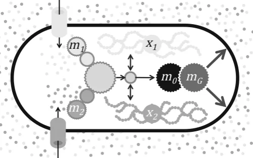
Fig. 1 Schematic representation of the model described by the system (8) for the casen=2. Two types of nutrients are assimilated by dedicated pathways (m1andm2) that feed into core metabolism from which building blocks are sluiced to machinery synthesis (m0) and growth (mG). Core metabolism also exchanges

molecular building blocks with reserves (x1andx2)

and the response measured in terms of cellular composition, cellular density, as well as consumption and production of relevant chemical species (e.g.,de Wit et al. 1995). The present paper describes the basic structure of VIS-plus-reallocation models, taking care to distinguish fundamental stoichiometric principles such as mass con-servation from the constitutive relations that express the regulatory rules. We discuss the compatibility of this new class of models with well-established empirical laws in microbial growth and metabolism, as well as the observability of these constitutive relations. Moreover, we prove the uniqueness and stability of the equilibrium point under a reasonable assumption on the general appearance of the constitutive relations.

2 Variable internal stores plus dynamic allocation theory

The model consists of stoichiometric equations, which are based on standard chem-ical conservation principles, presented in Sect.2.1, and constitutive relations, which express specific assumptions regarding the regulatory control pathways; one simple choice is discussed in Sect.2.2. A schematic representation of the model (forn =2) is given in Fig.1. Notation is summarised in Table1, and key simplifying assumptions are summarised in Table2.

2.1 Stoichiometric equations

2.1.1 Basic definitions and dynamics

Table 1 Notation employed in the equations describing the model

Symbol Biological interpretation Units

State unscaled variables

Mi C-molar amount ofi-type molecular

machinery

Moles of carbon

Xj Molar amount of the primary

elementXjin a reservej

Moles of the primary element in a reserve

W C-molar amount of the structural component

Moles of carbon

μ Specific growth rate Per unit of time State scaled variables

mi Density ofi-type molecular

machinery

Dimensionless

xj Density of a reservej Dimensionless

μ Specific growth rate Dimensionless Unscaled stoichiometric coefficients

φi The rate of production of the

machinery of typei

Units ofMiper unit ofM0per unit of time

φj i The gain of reservejper unit

machinery of typei

Units ofXjper unit ofMiper unit of time

σj W The loss of reservejfor growth Units ofXjper unit ofW

σj i The loss of reservejfor synthesis of

the machinery of typei

Units ofXjper unit ofMi

ψW The rate of production of the

structural component

Units ofWper unit ofMGper unit of time

Scaled stoichiometric coefficients

ψj i The gain of reservejper unit

machinery of typei

Dimensionless

σj i The loss of reservejfor synthesis of

the machinery of typei

Dimensionless

ψW The rate of production of the

structural component

dimensionless

Constitutive relationships

αi Portion of the zero machinery

devoted to the synthesis of machinery of typei

Dimensionless

ri Concentration of translationally

active mRNA for the machinery of typei

Units of concentration

ri Scaled variable for theri Dimensionless K Slope of the increasing part of the

piecewise functionrG

Dimensionless

Defines the interval on the abscissa for the increasing part of the piecewise functionrG

Table 1 continued

Symbol Biological interpretation Units

Miscellany

φi Maximum rate of the flux through the

assimilatory machinery of typei

Units of nutrient per unit ofMiper unit of time

fi Defines the ambient conditions for

the nutrienti

Dimensionless

R Chemical composition of the reserves as ann×nmatrix

N Chemical composition of the nutrients as ann×nmatrix

γj i (j,i)th element ofR−1·N Dimensionless

m Scaling parameter forM0/W Units ofM0per unit ofW for all subscriptsi,j :i∈ {0,1, . . . ,n,G},j∈ {1, . . . ,n}

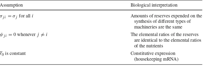
Table 2 Assumptions used in the analysis of the model

Assumption Biological interpretation

σj i=σjfor alli Amounts of reserves expended on the

synthesis of different types of machineries are the same ψj i=0 wheneverj=i The elemental ratios of the reserves

are identical to the elemental ratios of the nutrients

r0is constant Constitutive expression (housekeeping mRNA)

for all subscriptsi,j :i∈ {0,1, . . . ,n,G},j∈ {1, . . . ,n}

as intermediates of catabolic and anabolic pathways that are maintained at appropriate cellular concentrations by mechanisms not represented explicitly in the model. The C-molar amount of the structural component will be denoted asW.

Molecular machinery is divided inton+2 components, wherenis the number of

chemical species of nutrient for which we wish to account (this choice is informed by available data as well as the envisaged application of the theory). Components 1 through n represent the apparatus dedicated to the assimilation of the correspond-ing nutrients (transporters, bindcorrespond-ing proteins), in addition to the catalytic machinery that transforms these nutrients into core metabolites. Component 0 is the machinery

required to synthesise machinery. Component n+1, which will be given the

sub-script G, represents machinery devoted to growth, that is, the synthesis of the cell

envelope and duplication of the genome. The C-molar amounts of thesen+2 types

of machinery will be denoted asMi.

storage proteins, whereas others, such as sulphur globules and polyphosphate inclu-sions that contain no carbon (Preiss 1989), are expressed in terms of molar amounts of the primary element Xj. These Xj-molar amounts (where Xj is possibly but not

necessarily C) will be denoted asXj.

Although machinery is a heterogeneous assembly of proteins, nucleic acids, and co-factors (Neidhardt et al. 1990), it is nonetheless reasonable to assume that its chemical composition exhibits negligible fluctuations about the average typical of each kind of machinery. The dynamics of each component can then simply be written as follows:

˙

Mi =αiM0φi, (1)

wherei ∈ {0,1, . . . ,n,G},αi is an allocation coefficient indicating which portion

of the zero machinery is devoted to the synthesis of machinery of typei, andφi is

a stoichiometric coefficient. Parameters are indicated with a tilde to signify that they are dimensional; this allows the use of the same symbols when the model is rendered dimensionless (Sect.2.1.2). Being a fraction,αi is non-negative and subject to the

constraint

i∈{0,1,...,n,G}

αi =1. (2)

A unit of zero machinery spends a fractionαiof its time producingi-type machinery.

Thus, when αi = 1, every unit of time,φi units of machinery of typei are being

produced per unit of zero machinery. The reserve components change according to the balance of uptake and expenditures (Dawes 1989):

˙

Xj = n

i=1

ψj iMi −σj WW˙ −M0

i∈{0,1,...,n,G}

σj iαiφi, (3)

whereψj i is the gain of reserve jper unit machinery of typei,σj i is a

stoichiomet-ric coefficient for the synthesis of machinery of typei, andσj W is a stoichiometric

coefficient for growth. The last coefficient can be further analysed into an assimilatory component, i.e. reserve j is used as building block, and a dissimilatory component, i.e.jis used as energy source; in general, reservejmight be used in both ways andσj W

represents the net effect. Growth proceeds in proportion to the quantity of machinery that is dedicated to it:

˙

W =ψWMG, (4)

whereψW is a stoichiometric coefficient. The specific growth rate equalsW−1W˙.

LetφifiMi denote the flux of nutrient molecules through assimilatory machinery

of typei, whereφiis a maximum rate and fi ∈ [0,1]depends on ambient conditions

group or carbon skeleton that is not transformed by the metabolism of the organism of interest can be treated as an ‘element.’ For the sake of simplicity, we take the number of elements of interest to be equal to the number of reservesn. Nutrientihas chemical formulaEν(11)i, E

(2) ν2i E

(3) ν3i . . .E

(n)

νni, where the subscriptνkiis the number of elementkin

a molecule of nutrienti. The chemical composition of the nutrients can be collected in ann×nmatrixNwhoseith column is[ν1i, ν2i, ν3i, . . . , νni]T. Similarly, the chemical

composition of the reserves can be represented in ann×nmatrixRwhosejth column is the formula of reserve j. Inasmuch as reserve compounds are chemically distinct for different nutrients, we can assume that the inverseR−1exists. We then have an explicit expression for the stoichiometric coefficientψj i:

ψj i =γj iφifi, (5)

whereγj i denotes the(j,i)th element ofR−1·N.

2.1.2 Scaling

Choosing suitable parameters as natural units, we may render the equations dimen-sionless, which can facilitate the analysis of a mathematical model (van den Berg 2011). Adoptingφ₀−1as unit of time, we define scaled variables as follows:

mi =

Miφ0 Wmφi

; xj =

Xj

Wσj W.

(6)

Heremis a scaling parameter forM0/W; its significance will be discussed in Sect.2.2. Scaled stoichiometric parameters are defined as follows:

ψj i =

ψj iφim

σj Wφ02

; ψW =

ψWφGm

φ2 0

; σj i =σ j iφim

σj Wφ0

. (7)

On this scaling, the specific growth rate(Wφ0)−1W˙ is equal toψWmG; it is convenient

to give this quantity its own symbolμ. The biochemical similarity of different types of machinery implies that the relative amounts of reserves expended on their synthesis will be similar as well. This motivates the assumption that for every reservej, we have

σj i =σj for all machineriesi. The scaled state variables{m0, . . . ,mG,x1, . . . ,xn}

represent densities: these are intensive variables, as opposed to the original variables {M0, . . . ,MG,X1, . . . ,Xn}, which are extensive (i.e,∝ W). After scaling, we have

the following dynamics:

˙

mi =αim0−μmi for i ∈ {0,1, . . . ,n,G}

˙

xj = ni=1ψj imi−μ

1+xj

−m0σj for j∈ {1, . . . ,n}. (8)

For the sake of simplicity, we shall assume henceforth thatψj i =0 whenever j =i.

R−1·N will be diagonal. Choosing the elements of interest judiciously can also ensure that the matrixis diagonal. For instance, forE. coligrowing on glucose and ammonia, only the off-diagonal elements corresponding to hydrogen and oxygen are non-zero; focussing on only carbon and nitrogen, we obtain a 2×2 diagonal matrix.

2.2 Constitutive relationships

To complete the specification of the model, we require expressions for the allocation coefficientsα0, . . . , αG. One option is to treat these as forcing functions that drive the

model. These functions can be observed directly, due to recent advances in ribosome profiling (Ingolia et al. 2009;Li et al. 2014) and enzyme re-profiling (Kramer et al. 2010). Alternatively, the allocation coefficients can be treated as control inputs, to be calculated on the basis of a suitable, evolutionarily relevant optimality criterion (van den Berg et al. 1998). Another option to ‘close’ the equations is to posit outright the dynamics for the reserve densitiesxi, for instance settingx˙i =νi(fi−xi), whereνiis

a positive constant (Kooijman 2009) and fias in Eq. (5). This approach, which defines

the allocation implicitly, while having the advantage of simple dynamics, would seem to require cellular-level stoichiometric parameters to be in fortuitous agreement with the kinetic parameters of the molecules of the regulatory system (van den Berg 1998a). Here, we treat the allocation coefficients as a function of the internal state variables and/or environmental parameters (Parnas and Cohen 1976). In particular, we assume that m0, . . . ,mG,x1, . . . ,xn are mapped to α0, . . . , αG by a suitable R2(n+1) →

R2(n+1) _{function. Recalling thatα}

i is the fraction of ribosome time devoted to the

production of machinery of typei, we propose the following:

αi =

ri

r0+r1+ · · · +rn+rG,

(9)

where theri represent, roughly speaking, the concentrations of translationally active

mRNA for the corresponding types of machinery (corrected for relevant molecular properties, such as affinity for the ribosome and mobility within the cytosol, which we tacitly assume can be done via suitable weighting coefficients; synthesis rates in

E. coliare predominantly under translational, rather than transcriptional control (Li et al. 2014). For the sake of simplicity,r0is assumed to be constant, corresponding to constitutive expression. We scale the otherri by this constant:

ri =ri/r0. (10)

Forj =1, . . . ,n,rjis assumed to be a decreasing function ofxj(we shall take this as

time (cf. the Scott-Hwa-model;Scott et al. 2010, 2014;Scott and Hwa 2011). The

rj can be thought of as corresponding to levels of mRNA for the various types of

molecular machinery, although issues such as differences in stability of the mRNA molecule, affinity for ribosomes may distort a direct 1-to-1 correspondence (which can be compensated to some extent by assuming that appropriate correction factors have been assimilated into the scaling).

We assume further thatrGis an increasing function ofm0. For the sake of simplicity,

we represent it as a piecewise affine function:

rG[m0] =

⎧ ⎨ ⎩

0 if m0≤1−

rG,max/2+K(m0−1) if 1− <m0≤1+

rG,max if m0>1+,

(11)

where K is the slope, and = rG_,max/(2K). The midpoint of this function is set

atm0 = 1 (we here exercise our freedom to choose a natural unit for the scaling

factormwhich we identify as the physiological optimum for type-zero machinery;

m0 = 1 follows from this choice). Equation (11) expresses the hypothesis that the

safeguarding of core catalytic machinery takes precedence over growth (Bleecken

1988). This relationship is suggested by, and consistent with,Herbert(1961) classic observations on the relationship between RNA content and growth rate (the component

m0corresponding to rRNA). The slope of the relationship observed byHerbert(1961) is inversely proportional toK, that is, the larger the value ofK, the smaller the variation of RNA content with growth rate.

3 Consistency with classic models; observability

In this section we investigate the casen =1 in more detail, with an emphasis on the continuity of the present approach with the classic empirical laws proposed byMonod (1949) andDroop(1968). In addition, we discuss how the functionr1can be observed by transforming available observational data in a suitable way. This is important since ther-functions are the only non-standard (and possibly controversial) constituents of the model, as its remaining assumptions are closely linked to the law of conservation of mass.

3.1 Equilibrium conditions forn=1

System (8) takes on the following form forn =1:

˙

m0=α0m0−μm0; ˙m1=α1m0−μm1;

˙

mG =αGm0−μmG; ˙x1=ψ1m1−μ (1+x1)−σ1m0, (12)

with allocation fractions

α0=

1

1+r1+rG; α1=

r1

1+r1+rG; αG =

rG

At equilibrium, the rates of change in system (12) equal zero, which can be reduced, via the considerations presented in Sect.5.1for generaln, to the following pair of equilibrium conditions:

μ=ψWrGm0=(1+rG+r1)−1 (13)

ψ1r1=ψWrG(1+x1)+σ1. (14)

Provided thatrG_,max is sufficiently large (which is biologically plausible) the state

variablem0 can be assumed to lie in the interval(1−,1+). We then have the boundsψ₁{+}< ψ1< ψ₁{−}andμ{−}< μ < μ{+}, where

ψ1{±}=

σ1 r1(x1)+

ψW(1+x1)

2r1(x1)

4

ψW(1±)+(

1+r1(x1))2−(1+r1(x1))

(15)

μ{±}=1 2

ψW(1±)

4+ψW(1±) (1+r1(x1))2

−ψW(1±) (1+r1(x1))

(16)

and we have writtenr1(x1)to emphasise thatr1is a function ofx1. For small, these bounds converge and Eqs. (15) and (16) furnish simple expressions for the steady-state relationships betweenψ1,μ, andx1; this limit obtains whenK is sufficiently large.

3.2 Observability of the functionr1(·)

Two constitutive functions remain to be specified: the dependence ofψ1on the ambient

concentration of the nutrient, and the functionr1(·). For the former, the Michaelis-Menten hyperbola is a standard choice (van den Berg 2011):

ψ1=ψ1

1+K_ψ,1/[N1] ₋1

, (17)

whereψ1andKψ,1are positive parameters and[N1]is the ambient nutrient

concen-tration.

The functionr1(·)can be recovered from observational data as shown in Fig.2, via the parametric dependence ofx1andr1onμat steady state. Under strict homeostasis of type-zero machinery (a condition which we will denote asm0=. 1) we have

x1=ψ1

μ−2_−μ−1_−ψ

W−1

−(1+σ1/μ) (18)

r1=μ−1−1−μ/ψW (19)

which means that the construction of Fig.2 can be carried out if the steady-state relationship betweenψ1andμis available. Equation (17) can be used to recover this

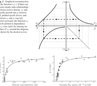
Fig. 2 Graphical reconstruction of the functionr1(·). If there are known steady-state relationships between reserve densityx1and specific growth rateμ(bottom left, printedupside down), and betweenr1andμ(top left, mirror reversed), the functionr1 can be plotted in dependence ofx1(top right) by chasing set values ofx1around the diagram, as shown by thedashed arrows

r

x

x

1

x

1

x

1

μ

μ

r

1

0 10 20 30 40 50

0.0 0.2 0.4 0.6 0.8

0.0000 0.0002 0.0004 0.0006 0.0008 0.0

0.2 0.4 0.6 0.8 1.0 1.2 1.4

Glucose concentration (M) Vitamin B12quota (10−12g/cell)

μ

(1/hour)

μ

(1/da

y

)

Fig. 3 Empirical laws.Leftsteady-state relationship between ambient nutrient concentration and specific growth rate.Escherichia colidata fromMonod(1949), together with the optimal non-linear least-squares fit of his model, Eq. (20):K_μ,1=6.39×10−5M;μ=1.45 h−1.Rightsteady-state relationship between cell quota and specific growth rate.Monochrysis lutheridata fromDroop(1968), together with the optimal non-linear least-squares fit of his model, Eq. (22):Q10=3.09×10−12g/cell;μ=0.835 day−1

an example of which is shown in Fig.3, which shows data obtained byMonod(1949) along with the hyperbola which he proposed as an empirical law:

μ=μ(1+K_μ,1/[N1])−1, (20)

whereμandK_μ,1are positive parameters andμis the measured specific growth rate in

an appropriate SI unit (by scaling,μ=μφ0). The resemblance to Eq. (17) is obvious,

although K_ψ,1 = Kμ,1(Button 1991);Monod(1949) pointed out that Kμ,1can be

one or several orders of magnitude smaller thanK_ψ,1.

not distinguishable as belonging to one or the other). However, it is always possible to observe the total amount per cell, known as thecell quota, which can be related to the components via a linear stoichiometric combination:

Q1=κW +κm,0m0+κm,1m1+κm,GmG+κx,1x1, (21)

where theκ account for the amount of nutrient that is incorporated per unit of the

corresponding component. An empirical law relatingQ1andμis known as aDroop

curve, afterDroop(1968) who proposed the following empirical relationship:

μ=μ (1−Q10/Q1) , (22)

whereμand Q10 are positive parameters (see Fig.3). In the special casem0 =. 1, Eqs. (21) and (22) yield:

x1= Q10/κx,1

1−μφ0/μ

− κm,1

κx,1μ+μ

κm,1−κm,G

κx,1ψW −

κW +κm,0−κm,1

κx,1

(23)

which furnishes the curve needed for the first transformation in Fig. 2(bottom left panel), the second transformation being given by Eq. (19), as before.

3.3 Strict reserve homeostasis and the transient Monod model

A case of special interest is that ofstrict homeostasis of the reserve x1. Let

r1=r1(1+exp{ϑ1(x1−ξ1)})−1, (24)

wherer1,ϑ1andξ1are positive parameters (any generic sigmoid function will do for

the purpose at hand). Consider the limitϑ1 → ∞; the function becomes infinitely

steep in the neighbourhood ofx1 = ξ1, so thatx1remains close toξ1over most of

the physiological range (excepting perhaps at low growth rates). We shall denote this special case as x1 =. ξ1. Combining this with Eq. (17) andm0 =. 1, we obtain the

following relationship between[N1]andμ:

ψ1/ (1+ξ1)

1+K_ψ,1/[N1] =

σ1/ (1+ξ1)+μ/φ0

φ0/μ−1−μ/(φ0ψW)

. (25)

This relationship has five free parameters, which is too many to be determined by least-squares fitting from Monod’s data in Fig.3alone, but good agreement with the data can be attained (in suitable limits for the parameters, the solution forμof Eq. (25) reduces to Monod’s hyperbola).

The ordinary differential equation

˙

W =Wμ1+K_μ,1/[N1] ₋1

is often referred to as the “Monod model” (e.g.,Dawes 1989;van Gemerden 1993;de Wit et al. 1995), where[N1]is treated as an autonomous function of time or coupled

toWvia a suitable ecological model (for instance, if the culture is growing under batch conditions,[N1]will decrease asWincreases). Equation (26) is more accurately called

thetransient Monodmodel to indicate that application to transient conditions ventures beyond the steady-state originally considered by Monod. The transient Monod model has just one component (W is its only state variable); when it occurs as part of an ecological model, stoichiometric consistency requires thatx1=. ξ1, so the assumption

of strict reserve homeostasis must be imputed to such studies even when the authors do not explicitly commit to this.

The behaviour of the present model under transient conditions differs from the transient Monod model, even under the assumption that the function r1(x1)has a steep slope (ϑ1→ ∞). Following a change in environmental conditions, for instance

a step change in[N1],x1deviates fromξ1which triggers a re-allocation of building

blocks to the various types of machinery. As[N1]is held constant at its new value, the m-type state variables relax at a time scale∼μ−1; whilex1relaxes back toξ1.

However, the transient Monod model and the present model can be treated as equivalent if the changes in [N1] (and hence ψ1) occur smoothly and sufficiently

slowly. In this ‘adiabatic’ case, the internal dynamics is sufficiently rapid that its state variables can be coupled quasi-statically to[N1], or, equivalently, toψ1(cf. Sect.4.1).

4 Simulations

The dynamics, system (8), can be studied in qualitative terms by means of numerical solution of the ordinary differential equations. In this section we note several aspects of the model’s dynamic behaviour which could be measured, in principle, in the real-life system.

4.1 The casen=1

The response of the model to stepwise increases and decreases ofψ1is shown in Fig.4.

It can be seen that the downward steps inψ1, representing a decrease in ambient nutrient

availability, lead to downward deflections in the reservex1which governs the dynamic allocation between nutrient uptake machinery and proliferative (growth) machinery. The adjustment is rapid and stabilises, although oscillations become more vigorous and long-lasting at lower values of ψ1; intuitively this can be understood since the

actual balance betweenm1andmG (i.e., the proteome-level profile) relaxes toward

the balance dictated byα1andαGwith a response time of orderμ−1. Thus, even if the

change in expression of different kinds of machinery is rapid, the actual balance reacts more sluggishly at lowμ. Upward step changes inψ1induce upward deflections ofx1,

which again steer the dynamic re-allocation process.

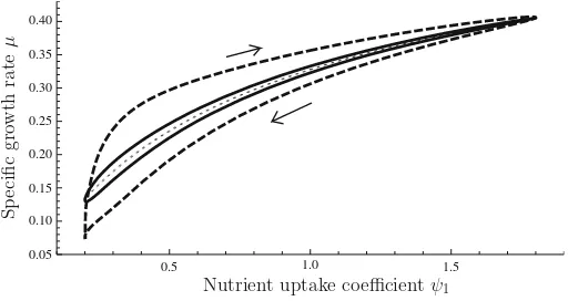
If a sinusoidal variation inψ1is imposed, the system settles on a stationary cycle.

Parametric plots ofψ1(t)versusμ(t)over this stationary cycle are shown in Fig.5

0 20 40 60 80 1.0

1.5 2.0

20 40 60 80

1.0 1.1 1.2 1.3 1.4 1.5

0 20 40 60 80

0.1 0.2 0.3 0.4 0.5 0.6

ψ1

x1

μ

Scaled timet

Fig. 4 Numerical solution of system (12). The functionrGwas as in Eq. (11) withK=104andrG,max=5;

r1=15/ (1+exp{10(x1−1)});ψW =1; andσ1=1.Topimposed time course ofψ1.Middletime course

of scaled reserve densityx1.Bottomtime course of the specific growth rateμ

0.5 1.0 1.5

0.05 0.10 0.15 0.20 0.25 0.30 0.35 0.40

Sp

ecific

gro

wth

rate

μ

Nutrient uptake coefficientψ₁

Fig. 5 Numerical solution of system (12); stationary cycle under a sinusoidal variation ofψ1. Thedashed curveobtains for a cycle duration of 60 units of scaled time; thesolid curvefor a cycle duration of 300 units. Also shown is the ‘adiabatic’ limit (dotted line) which obtains for an infinitely slow cycle

behind the prevailing value ofψ1. The hysteresis loop widens as the period of the

environmental oscillation shortens. As this duration goes to infinity, the loop tight-ens up against a curve which corresponds to the ‘adiabatic’ regime under which the transient Monod model is valid: provided that environmental changes are sufficiently slow,μcan be treated as a function of the environmental conditions.

4.2 The casen=2

For two or more reserve components, the assumption of monotonically decreasingri

-functions leads to a re-balancing effect, whereby stoichiometric imbalances between nutrient availabilities are offset, or at least partially offset, by counteracting changes in the allocation fractions to the corresponding types of uptake machinery.

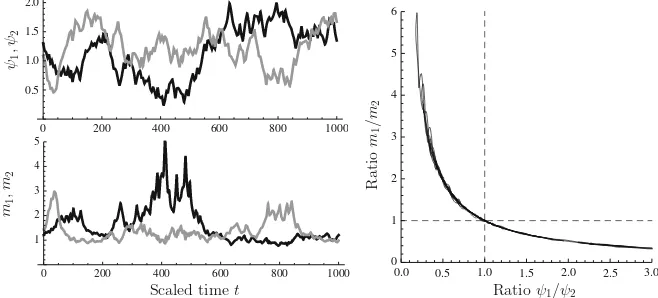
This ‘counter-skewing’ effect is illustrated in Fig.6, in which the model was simu-lated forn=2 with uncorrelated white noise in theψ1andψ2time-courses. It can be

0 200 400 600 800 1000 0.5

1.0 1.5 2.0

0 200 400 600 800 1000 1

2 3 4 5

0.0 0.5 1.0 1.5 2.0 2.5 3.0

0 1 2 3 4 5 6

ψ1 ,ψ2

m1

,m

2

Scaled timet Ratioψ₁/ψ₂

Ratio

m1

/m

2

Fig. 6 Numerical solution of system (8) withn=2. The functionrG was as in Eq. (11) withK =104

andrG,max=5;ri=15/ (1+exp{10(xi−1)})andσi=1 fori=1,2; andψW =1.Left,topimposed

time course ofψ1(black line) andψ2(grey line).Left,bottomtime course of scaled uptake machinery for nutrient 1 (m1;black line) and nutrient 2 (m2;grey line). Right:ψ1/ψ2versusm1/m2, showing compensatory shifts in expression of nutrient uptake machinery

the ratioψ1/ψ2is plotted againstm1/m2over the time course of the simulation run,

a perfect hyperbola is obtained.

The model achieves this behaviour by having each reserve feeding back on the expression of the machinery feeding that particular reserve; the balancing in allocation happens at the level of Eq. (9), which represents the effect of ribosomes distributing themselves pro rata over the mRNA species, as we would expect based on the random encounter processes that underlie molecular kinetics. This shows that it is possible in principle to achieve reserve homeostasis without the need for signals arising from multiple reserves to converge on the upstream activation sequence of any one of the genes for uptake machinery.

4.3 Multiple reserve components

The qualitative behaviours noted in the foregoing sections are also present atn ≥3. By way of example, the response of a model withn=12 is shown in Fig.7. Again, the ambient medium presents uncorrelated noise. The response to this environmental input is represented for four different steepness values [ϑi, see Eq. (24)] of theri-functions.

When this value is low, the allocation to the uptake machineries is hardly adjusted. As a result, the entropy of the reserves follows that of the environment; in other words, the fluctuations in the environment are reflected in fluctuations in reserve status (in the simulation shown forϑi =0.2, the reserve entropy temporarily undershoots the

ambient entropy; this is a transient effect due to the initial state of the system).

Asϑi increases, the reserve entropy tends more and more toward the maximum

0 200 400 600 800 1000 4

6 8 10

0.0 0.5 1.0 1.5 2.0

0.2 0.4 0.6 0.8 1.0

Scaled timet Scaled reserve densityxi ri

ψi ϑi= 20

ϑi= 2

ϑi= 0.2

ϑi= 0.5

0 200 400 600 800 1000

2.38 2.40 2.42 2.44 2.46 2.48

0 200 400 600 800 1000

2.38 2.40 2.42 2.44 2.46 2.48

0 200 400 600 800 1000

2.38 2.40 2.42 2.44 2.46 2.48

0 200 400 600 800 1000

2.38 2.40 2.42 2.44 2.46 2.48

ϑi= 0.2

ϑi= 0.5

ϑi= 2

ϑi= 20

0 200 400 600 800 1000

0.002 0.004 0.006 0.008 0.010 0.012 0.014

0 200 400 600 800 1000

0.002 0.004 0.006 0.008 0.010 0.012 0.014

0 200 400 600 800 1000

0.002 0.004 0.006 0.008 0.010 0.012 0.014

0 200 400 600 800 1000

0.002 0.004 0.006 0.008 0.010 0.012 0.014

ϑi= 0.2

ϑi= 0.5

ϑi= 2

ϑi= 20

Scaled timet

En

trop

y

Scaled timet

Fig. 7 Numerical solution of system (8) withn =12, with initial condition corresponding to optimal environment, i.e.,ψi ≡ψifor alli.Top leftuncorrelated white noise functions forψi(i =1, . . . ,12)

used in all simulations.Top rightsigmoid functions used forriin the simulations; all reserves use the same

function in any given run, but the steepness parameterϑiwas varied as shown.Bottom lefttime course of the

reserve entropy (solid line) for various values ofϑi; the input entropy of theψiis shown for reference as a grey line. Reserve entropy was defined as n_i=1(xi/xT)ln{xT/xi}withxT= ni=1xi; Ambient entropy

was defined as n_i=1(ψi/ψT)ln{ψT/ψi}withψT = ni=1ψi.Bottom righttime course of the

rela-tive entropy for various values ofϑi; relative entropy was defined as ni=1(mT/mi)ln{mTψT/(miψi)}

withmT= ni=1mi

rather restless, with rapid downward spikes that arise as a consequence of the high reactivity of the feedback loop, which tends to induce rapid oscillations.

To visualise the ‘counter-skewing’ effect, the relative entropy of {m−_i 1}n_i=1 with respect to{ψi}n_i=1has been plotted as a function of time. This relative entropy decreases

with increasingϑi, indicating that the machinery allocation becomes better adapted

to the environmental fluctuations. Again, the trace forϑi =20 appears more agitated

than that forϑi =2, due to the rapid oscillations concomitant with high reactivity.

5 Dynamics of the model for general

n

We investigate the existence, uniqueness, and stability of equilibria of system (8). Setting the rates of change equal to zero yields the equilibrium conditions:

αim0−μmi =0 for i ∈ {0,1, . . . ,n,G}, (27)

ψjmj−μ

1+xj

We shall assume throughout thatis a diagonal matrix, and we are primarily interested in the case whereK is large (corresponding to strict homeostasis ofm0).

5.1 Existence and uniqueness of the equilibrium point

Specifying Eq. (27) fori = 0, we obtainμ =α0 (sincem0 >0 for a biologically

relevant equilibrium). Thus Eq. (27) can be written asmi =(αi/α0)m0. With Eq. (9),

this becomesmi =(ri/r0)m0ormi =rim0sincer0 ≡1 by scaling. In particular,

mG =rGm0and henceμ=ψWrGm0(sinceμ=ψWmGby definition). With these

identities, Eq. (28) becomes:

ψjrj−ψWrG

1+xj

−σj

m0=0,

which means that eitherm0=0, which is not biologically relevant, or

ψWrG

1+xj

+σj =ψjrj. (29)

Let us first consider the problem of solving this forxj given a fixed value ofrG ∈

[0,rG,max]. The left-hand side of Eq. (29) is a strictly increasing function ofxjwhereas

its right-hand side is a strictly decreasing function ofxj(by the assumed properties of

therj as functions of thexj). The graphs of these two functions intersect in at most

one point. This point will exist if the graph of the left-hand side of Eq. (29) lies below that of the right-hand side atxj =0. For this it suffices that

rj,max≥

ψWrG,max+σj

/ψj, (30)

where rj,max denotes the value of rj at xj = 0. The physiological interpretation

suggests thatrj,max < +∞, so that condition (30) can only be satisfied ifψj > 0

for j =1, . . . ,n. Thus, if condition (30) is satisfied, Eq. (29) will have a unique solu-tionx_j ≥0 for all reserves j, for the given value ofrG. This solutionx_j can be treated

as a function ofrGas defined by Eq. (29); this function is strictly decreasing. Since the

rjare strictly decreasing in their respectivexj, it follows that r≡ j_∈0_,1_,...,n_,Grj

is an increasing function ofrG. At equilibriumμ=α0andα0=r0/ r=1/ r,

whenceμ=1/ rwhich is a decreasing function ofrG, or equivalently, a decreasing

function ofm0(sincerGis an increasing function ofm0). In addition,μ=ψWrGm0,

which is an increasing function ofm0. Again we consider the point of intersection between the graphs of these two functions. Repeating a similar argument, we find that 1/ r>0 andψWrGm0=0 atm0=1−, and that therefore it is sufficient if

⎛

⎝1+rG,max+

n

j=1

r_j(rG,max) ⎞

⎠_ψWrG,max≥(1+)−1 (31)

are fixed whenever thexjtogether withm0are fixed. Conditions (30) and (31) suffice;

they could be weakened but even in the form stated, they are not at all stringent from a biological point of view: it is enough that therj-functions are sufficiently large for

small values of their argument. We henceforth assume that these conditions are met.

5.2 Linear stability analysis

We investigate the stability by linearising the system about its equilibrium and verifying the stability of the characteristic polynomial associated with the linearised system. The system matrix of the linearised system is the Jacobian matrix:

J(m0,m1. . .mn,mG,x1. . .xn)

= ⎛ ⎜ ⎜ ⎜ ⎜ ⎜ ⎝

∂f1

∂m0

∂f1

∂m1 . . .

∂f1

∂mn

∂f1

∂mG

∂f1

∂x1 . . .

∂f1

∂xn

∂f2

∂m0

∂f2

∂m1 . . .

∂f2

∂mn

∂f2

∂mG

∂f2

∂x1 . . .

∂f2

∂xn

... ... ... ... ... ... ... ...

∂f2n+2

∂m0

∂f2n+2

∂m1 . . .

∂f2n+2

∂mn

∂f2n+2

∂mG

∂f2n+2

∂x1 . . .

∂f2n+2

∂xn

⎞ ⎟ ⎟ ⎟ ⎟ ⎟ ⎠,

where f1, f2. . . f2n+2denote the right-hand sides of system (8). Our strategy is to

investigate the signs of the coefficients in the limit K → ∞[the parameterK rep-resents the slope of the increasing part of the piece-wise functionrG in Eq. (11)].

In real-life systems, K < +∞, as attested by the non-zero slope of cellular RNA

content (∼m0) as a function ofμat steady state (Herbert 1961). In other words, the

limit K → ∞represents an idealised case of strict homeostasis ofm0. While our

limiting result establishes that stability is ensured ifK is sufficiently large, numerical solutions of the dynamic equations for finiteKindicate that, in fact, the system always converges to its equilibrium point, but, asKdecreased, with oscillations of increasing amplitude and ring-down time. To establish the result in the limitK → ∞, we exploit

a theorem byStrelitz(1977) on the stability of monic polynomials.

5.2.1 Signs of the coefficients of the characteristic equation

The characteristic equation is a polynomial of order 2(n+1):

λ2n+2₊

c1λ2n+1+c2λ2n+ · · · +c2n+1λ+c2n+2=0. (32)

The coefficientsck can be written as ck = (−1)kSk, where Sk is the sum of the

principal minors Mk (Mishina and Proskuryakov 1962). These Mk are symmetric

with respect to the main diagonal of the Jacobian matrix. The coefficientsckare

first-order polynomials inK. For sufficiently largeK, it is the term inckthat is proportional

toK that governs the sign; letckdenote this term.

It will prove useful to partition the Jacobian matrix as follows:

The submatrices are evaluated at the equilibrium point in the limitm0→ 1, that is,

→0 [which obtains asK → ∞, cf. Eq. (11)]:

JI= ⎛ ⎜ ⎜ ⎜ ⎜ ⎜ ⎜ ⎜ ⎜ ⎜ ⎜ ⎜ ⎜ ⎜ ⎝

−ψ2

WK r

2

G

ψWr1rG−ψW2r1K rG2

...

ψWrnrG−ψ_W2rnK r_G2

ψWK rG+ψWrG2 −ψW2 K rG3

−σ1

...

−σn

⎞ ⎟ ⎟ ⎟ ⎟ ⎟ ⎟ ⎟ ⎟ ⎟ ⎟ ⎟ ⎟ ⎟ ⎠ ,

JII= ⎛ ⎜ ⎜ ⎜ ⎜ ⎜ ⎜ ⎜ ⎜ ⎜ ⎜ ⎜ ⎜ ⎝

0 . . . 0

−ψWrG . . . 0

... ... ...

0 . . . −ψWrG

0 . . . 0

ψ1 . . . 0

... ... ...

0 . . . ψn

⎞ ⎟ ⎟ ⎟ ⎟ ⎟ ⎟ ⎟ ⎟ ⎟ ⎟ ⎟ ⎟ ⎠

, JIII = ⎛ ⎜ ⎜ ⎜ ⎜ ⎜ ⎜ ⎜ ⎜ ⎜ ⎜ ⎜ ⎜ ⎜ ⎝

−ψW

−ψWr1

...

−ψWrn

−2ψWrG

σ1−ψ1r1

rG

...

σn−ψnrn

rG ⎞ ⎟ ⎟ ⎟ ⎟ ⎟ ⎟ ⎟ ⎟ ⎟ ⎟ ⎟ ⎟ ⎟ ⎠ ,

JIV= ⎛ ⎜ ⎜ ⎜ ⎜ ⎜ ⎜ ⎜ ⎜ ⎜ ⎜ ⎜ ⎜ ⎜ ⎝

−ψ2

Wr1rG2 . . . −ψW2rnrG2

ψWr₁rG−ψ_W2r1r₁r_G2 . . . −ψ_W2r1rnrG2

... ... ...

−ψ2

Wr1rnrG2 . . . ψWrnrG−ψ_W2rnrnrG2

−ψ2

Wr

3

Gr1 . . . −ψ 2

Wr

3

Grn

−ψWrG . . . 0

... ... ...

0 . . . −ψWrG

⎞ ⎟ ⎟ ⎟ ⎟ ⎟ ⎟ ⎟ ⎟ ⎟ ⎟ ⎟ ⎟ ⎟ ⎠ .

Lemma 1 Only the minors that contain a diagonal element from JIcontribute terms that are proportional to K ; in particular,

ck =C2kn−+11Kψ

k+1

W r k+1

G +C k−2 2n Kψ

k Wr

k−1

G

+

n

=1

C₂k_n−₋(2₍₂+₋1)₁₎Kψ_Wk+1−r_Gk−(−1)

×

S∈P({1,2...,n})

m∈S

r_m ⎛ ⎝rG

m∈S

ψm+

m∈S

(ψmrm−σm)

j∈S\m

ψj ⎞ ⎠ + n =1

C₂k_n−₋(2₂+2)Kψ_Wk−r_Gk−−1(−1) S∈P({1,2...,n})

m∈S

whereP({1,2. . . ,n})is the set of all subsets of the set{1,2. . . ,n}with cardinal-ity.

For example, forn =2 andk=6 we have:

c6=KψW7rG7 +KψW6rG5

−Kψ_W6r_G5r₁

ψ1rG+(ψ1r1−σ1)

−Kψ_W6r_G5r₂

ψ2rG+(ψ2r2−σ2)

+Kψ_W5r_G4r₁r₂

ψ1ψ2rG+ψ1(ψ2r2−σ2)+ψ2(ψ1r1−σ1)

−KψW5rG4ψ1r1−KψW5rG4ψ2r2+KψW4rG3ψ1ψ2r1r2. (35)

Proof Only the minors that contain a diagonal element from the first column contribute terms proportional toK, because the minors that do not contain elements fromJIdo not contain any term∝ K. There are 2n−1 non-trivial subsets of the set of sizen. To obtain all minors that contribute terms∝ K we have to inspect 23−1 =7 types of minor containing a diagonal element taken fromJI, as the ways in which such minors can be composed depends on the number of non-trivial subsets of the set of size 3. One of these types only occurs fork =2 (minors based on JIand JIII) and can be subsumed under type iii. This leaves six types to be distinguished; they are defined as being composed of the following, in addition to the element contributed by the column matrixJI_{: (i)k−1 diagonal elements fromJ}II_{; (ii)k−1 diagonal elements fromJ}IV_;

(iii)k−2 diagonal elements fromJIIand one fromJIII; (iv)k−2 diagonal elements from JIVand one from JIII; (v) diagonal elements fromJIIand JIVsuch that their total number isk−1; (vi) diagonal elements from JIIand JIV such that their total number isk−2, in addition to an element from JIII.

We consider these types in terms and collect the terms proportional toK. For the sake of clarity, expressions such as(−1)k−2, (−1)k−4etc. will be written as(−1)kand likewise(−1)k−1, (−1)k−3etc. will be written as(−1)k+1. The binomial coefficient _n

k

=n!(k!(n−k)!)−1will be denoted asCnk. We will make use of the following:

k

i₌0

C_niC_nk−i =C₂k_n and C_nk+C_nk−1=C_nk₊₁. (36)

Minors of type i have the following form:

−ψ2

WK rG2 0 . . . 0

ψWr1rG−ψ_W2r1K r_G2 −ψWrG . . . 0

... ... ... ...

ψWrk−1rG−ψ_W2rk−1K r_G2 0 . . . −ψWrG

=(−1)kKψWk+1r k+1

G .

We haveCnk−1such minors, because the first columnJIis fixed and we are choosingk−

1 diagonal elements from a total ofnelements in block JII. Thus minors of this type contribute(−1)kCnk−1KψWk+1r

k+1

Minors of type ii have the following form:

−ψ2

WK rG2 −ψW2r1rG2 . . . −ψW2rk−1rG2

−σ1 −ψWrG . . . 0

... ... ... ...

−σk−1 0 . . . −ψWrG

=(−1)kKψWk+1r k+1

G + · · · .

where the dots (here and in what follows) correspond to terms that do not containK. We haveC_nk−1such minors, giving a contribution(−1)kC_nk−1Kψ_Wk+1r_Gk+1to Eq. (34).

Minors of type iii have the following form:

−ψ2

WK r

2

G 0 . . . 0 −ψW

ψWr1rG−ψW2r1K rG2 −ψWrG . . . 0 −ψWr1

... ... ... ... ...

ψWrk−2rG−ψW2rk−2K rG2 0 . . . −ψWrG −ψWrk−2

ψWK rG+ψWr_G2 −ψ_W2 K r_G3 0 . . . 0 −2ψWrG

=(−1)k

Kψ_Wk+1r_Gk+1+(−1)kKψ_Wkr_Gk−1+ · · ·.

We have C_nk−2 such minors and the contribution is therefore (−1)kC_nk−2

Kψ_Wk+1r_Gk+1+Kψ_Wkr_Gk−1

.

Minors of type iv have the following form:

−ψ2

WK rG2 −ψW −ψW2r1rG2 . . . −ψW2rir2G . . . −ψW2rk−2rG2

ψWK rG+ψWr2G−ψW2K rG3 −2ψWrG −ψW2r1rG3 . . . −ψW2rirG3 . . . −ψW2rk−2rG3

−σ1 (σ1−ψ1r1)/rG −ψWrG . . . 0 . . . 0

..

. ... ... ... ... ... ...

−σi (σi−ψiri)/rG 0 . . . −ψWrG . . . 0

..

. ... ... ... ... ... ...

−σk−2 (σk−2−ψk−2rk−2)/rG 0 . . . 0 . . . −ψWrG

.

These contribute the same term as minors of type iii, i.e.

(−1)k_Ck−2

n

Kψ_Wk+1r_Gk+1+Kψ_Wkr_Gk−1

. In addition, minors based on the

diago-nal element of columni in block JIVcontribute(−1)kr_i(σi −riψi)KψWkr k−1

G . For

each i, there areC_nk−₋3₁ ways of making up the remaining k −3 elements (which are chosen from a total n −1 in block JIV). This yields a total contribution of

(−1)k_Ck−3

n−1 i_∈P1({1,2...,n})r

i(σi−riψi)Kψ k Wr

k−1

Minors of type v have the following form:

−ψ2

WK r2G 0 . . . 0 −ψW2r1rG2 . . . −ψ2Wrk−1−irG2

ψWr1rG−ψW2r1K rG2 −ψWrG . . . 0 ψWr1rG−ψW2r1r1rG2 . . . −ψ

2

Wr1rk−1−ir

2

G

..

. ... ... ... ... ... ...

ψWrirG−ψW2riK rG2 0 . . . −ψWrG −ψW2rir1r2G . . . ψW2rirk−1−irG2

−σ1 ψ1 . . . 0 −ψWrG . . . 0

..

. ... ... ... ... ... ...

−σk−1−i 0 . . . 0 0 . . . −ψWrG

.

Each minor contributes a term(−1)kKψ_Wk+1r_Gk+1. Since we are choosingk−1 diagonal

elements from blocksJIIandJIV, the multiplicity is k_i=−₁2CniCnk−1−i, giving a total

(−1)k k−2

i₌1CniCnk−1−iKψWk+1r k+1

G . Furthermore, each minor containing diagonal

elements from columniinJIIand columniinJIV, contributes(−1)k+1ψir_iKψ_Wkr_Gk.

There are _ik₌−₀3C_ni₋₁C_nk₋−₁3−i such minors, since for eachi we are choosingk−3 diagonal elements fromJIIand JIVcombined. Using k_i=−₀3C_ni₋₁C_nk−₋3₁−i =C₂k_n−₋3₂, we obtain

(−1)k₊1

Ck_2n−₋3₂

i∈P1({1,2...,n})

ψiriKψ k Wr

k G

as the total contribution to the right-hand side of Eq. (34). Next, given a pair(i,j)

withi = j, we consider minors containing diagonal elements from columnsiand j

inJIIand columnsiandjinJIV; such a minor contributes(−1)kr_ir_jψiψjKψWk−1r k−1

G .

The multiplicity is k_i=−₀5C_ni₋₂C_nk₋−₂5−i, since for a given choice(i,j)there remaink−5 elements to be chosen. Summing over all such pairs(i,j)and using the combinatorics formulae, Eq. (36), we obtain

(−1)k

C₂k_n−₋5₄ (i,j)∈P2({1,2...,n})

r_ir_jψiψjKψWk−1r k−1

G .

Next, after pairs of columns, we need to consider triples (i,j,k), and so on. The

general formula for an-tuple can be obtained via similar reasoning, and summing

over all such tuples we obtain

(−1)k n

=1 ⎛

⎝C₂k−_n−(2₂+1)Kψ_Wk+1−r_Gk+1−(−1) S∈P({1_,2_...,n_})

m∈S

ψmrm

⎞ ⎠

as the final contribution.

Minors of type vi contain contributions from all blocks of the Jacobian matrix, cf. Eq. (33). Each minor contributes(−1)k k−3

i₌1CniCnk−2−iKψWk

ψWr_Gk+1+r_Gk−1

,

In analogy to type iv, minors of type vi contribute the following term∝K:

(−1)k k−3

q=1

CnqCnk−−31−q

i∈P1({1,2...,n})

r_i(σi −riψi)KψWk r k−1

G

and in analogy to type v, minors of type vi contribute the following term∝K:

(−1)k n

=1 ⎛

⎝C₂k−_n−(2₂+2)Kψ_Wk+1−r_Gk+1−(−1) S∈P({1_,2_...,n_})

m∈S

ψmrm

⎞ ⎠_.

There are further terms contributed by minors containing diagonal elements from columnsi and j in block JIV(wherei = j) in addition to a diagonal element from either columnsiorjin blockJII_{; such minors contribute(−1)}k+1_r

irj

ψi(ψjrj−σj)

+ψj(ψiri−σi)

Kψ_Wk−1r_Gk−2. Summing over all pairs(i,j)and using the combina-torics formulae, Eq. (36), we obtain

(−1)k+1

C₂k_n−₋5₃Kψ_Wk−1r_Gk−2 (i,j)∈P2({1,2...,n})

r_ir_jψi(ψjrj−σj)+ψj(ψiri−σi)

.

Next we consider triples(i,j,p), withi = j = p, and minors that take diagonal elements from columnsi,j, andpfrom blockJIVwhile blockJIIcontributes diagonal elements from a pair of columns, which is either the pair(i,j), or(i,p), or(j,p). Summing over all triples(i,j,p)and using the combinatorics formulae, Eq. (36), we obtain

(−1)kC₂k−_n−7₅ (i,j,p)∈P3({1,2...,n})

r_ir_jr_p

ψiψp(ψjrj−σj)

+ψjψp(ψiri −σi)+ψiψj(ψprp−σp)

Kψ_Wk−2r_Gk−3.

Generalising this argument to-tuples of columns chosen from JIV, we obtain the following:

(−1)k n

=2

C₂k−_n−(2₍₂+₋1)₁₎Kψ_Wk+1−r_Gk−(−1)

×

S∈P({1,2...,n})

m∈S

r_m ⎛

⎝

m∈S

(ψmrm−σm)

j∈S\m

ψj

⎞ ⎠_.

A term (−1)k+1ψir_iKψ_Wk−1r_Gk−2 is contributed by each minor that takes diagonal

multiplicity k_i=−₀4C_ni₋₁C_nk−₋4₁−i and simplifying the sum, we obtain

(−1)k₊1

C₂k_n−₋4₂

i∈P1({1,2...,n})

ψiriKψ k−1

W r k−2

G .

For a given pair(i,j), withi = j, minors taking diagonal elements from columnsiand

jinJII_{and from columnsiandjinJ}IV_{contribute(−1)}k_r

irjψiψjKψ k₋2

W r k₋3

G each.

The multiplicity of such minors is _ik₌−₀6C_ni₋₂C_nk−₋6₂−i. Summing over all pairs(i,j)

and simplifying, we have

(−1)kC₂k_n−₋6₄ (i,j)∈P2({1,2...,n})

r_ir_jψiψjKψ_Wk−2r_Gk−3.

Generalising to-tuples, we obtain

(−1)k n

=1

C₂k_n−₋(2₂+2)Kψ_Wk−r_Gk−−1(−1) S∈P({1,2...,n})

m_∈S

ψmrm.

Equation (34) is obtained by collecting terms proportional toK. In particular, terms∝

Kψ_Wk+1r_Gk+1have the following coefficients:

(−1)k

Ckn−1+(−1)kCnk−1+(−1)kCnk−2+(−1)kCnk−2

+(−1)k k−2

i=1

C_niC_nk−1−i +(−1)k

k−3

i=1

C_niC_nk−2−i

=(−1)k

_k−2

i=0

CinCnk−1−i+ k−3

i=0

CniCnk−2−i +Cnk−1+Cnk−2

=(−1)k

C₂k_n−1−C_nk−1+C₂k_n−2−C_nk−2+C_nk−1+C_nk−2

=(−1)k

C₂k_n−1+C₂k_n−2

=(−1)k

C₂k_n−₊1₁;

terms∝ Kψ_Wk r_Gk−1have the following coefficients:

(−1)k

C_nk−2+(−1)kC_nk−2+(−1)k

k−3

i=1

C_niC_nk−2−i

=(−1)k

C_nk−2+

k−3

i₌0

C_niC_nk−2−i

=(−1)k

Cnk−2+Ck2n−2−C k−2

n

=(−1)k