Optimal design when outcome values are not missing at random

DOI 10.5705/ss.202016.0526 Complete List of Authors Kim May Lee

Robin Mitra and Stefanie Biedermann,

Corresponding Author Kim May Lee

OPTIMAL DESIGN WHEN OUTCOME VALUES

ARE NOT MISSING AT RANDOM

Kim May Lee, Robin Mitra and Stefanie Biedermann

University of Southampton, UK

Abstract: The presence of missing values complicates statistical analyses. In design of experiments, missing values are particularly problematic when con-structing optimal designs, as it is not known which values are missing at the design stage. When data are missing at random it is possible to incorporate this information into the optimality criterion that is used to find designs; Imhof, Song, and Wong (2002) develop such a framework. However, when data are not missing at random this framework can lead to inefficient designs. We investigate and address the specific challenges that not missing at random values present when finding optimal designs for linear regression models. We show that the op-timality criteria depend on model parameters that traditionally do not affect the design, such as regression coefficients and the residual variance. We also develop a framework that improves efficiency of designs over those found when values are missing at random.

1. Introduction

Missing values are a common problem in many fields. Their presence

complicates statistical analysis, and appropriate methods are required to

handle the missing data to ensure valid inferences. There is a wide variety

of techniques to handle missing values once the data are observed, but the

objective in this paper is to focus on handling the missing data problem

at the design stage of an experiment. By incorporating information about

the missing data mechanism we may be able to design a more efficient

experiment that allows more information to be obtained from the data

collected.

There has been work on finding optimal designs for experiments with

potentially missing. The majority of the contributions is concerned with

robustness of designs to missing values; see for example Hedayat and John

(1974), Ghosh (1979), Ortega-Azurduy, Tan, and Berger (2008), and

Ah-mad and Gilmour (2010). Herzberg and Andrews (1976) and Hackl (1995)

introduce design criteria that account for the presence of missing responses

for some special cases. Imhof, Song, and Wong (2002) develop a framework

that finds optimal designs by taking the expectation of the information

ma-trix with respect to the missing data mechanism; this has been extended

covariance matrix.

These contributions to optimal design implicitly assume that the data

are missing at random, that the missing data mechanism depends on only

observed variables. This is referred to as a missing at random (MAR),

Ru-bin (1976). If it is assumed that the missing data mechanism depends on

unobserved variables, such as the missing values themselves, Rubin (1976)

referred to this as not missing at random (NMAR). Typically NMAR

prob-lems are much more challenging to handle, as learning about the exact form

of the NMAR mechanism is not typically possible, and thus often leads to

biased inferences.

To our knowledge there has not been any explicit consideration of

deal-ing with NMAR when finddeal-ing optimal designs. This article intends to

ad-dress the specific problems that NMAR causes in optimal design. We mean

to extend the framework of Imhof, Song, and Wong (2002) to incorporate

the possibility of NMAR, using an approximation to the bias. By doing

so we can mitigate the problems caused by NMAR and find more efficient

designs.

We assume that inferences stem from a linear regression model once the

experiment has been performed, and we deal with the missing data using

the context of regression analysis, complete case analysis can be appropriate

when the missing mechanism is MAR (Little (1992)). Under NMAR there

are obvious problems that can occur and these will be noted and mitigated

is our optimal design framework.

The remainder of the article is organised as follows. Section 2 presents

some background for the key elements of missing data and optimal design.

Section 3 motivates the problems NMAR causes in optimal design. Section

4 presents an optimal design framework that takes NMAR into account,

and compares how it relates to the traditional MAR framework. Section

5 empirically evaluates the proposed framework to determine the benefits

of using this approach. Section 6 evaluates our methodology in a data

scenario. Section 7 ends with some concluding remarks.

2. Background

We review the relevant background for dealing with missing data, then

present the key concepts in constructing optimal designs when a linear

regression analysis model is used, and we review how the potential for

missing data can be taken into account when finding optimal designs.

2.1 Missing data

Let xi, i= 1, . . . , n, represent a set of explanatory variables for unit i

is performed. We assume that inferences are drawn by fitting a linear

regression model to the data of the form,

y=Xβ+ (1)

wherey= (y1, . . . .yn),X is the design matrix,βis the vector of regression

coefficients and ∼N(0, σ2_{I) is the error vector with residual varianceσ}2_.

We define a missing indicator,mi, for each uniti;mi = 1 ifyiis missing and

mi = 0 otherwise. We write ymis ={yi : mi = 1} and yobs = {yi :mi = 0}

as the missing and observed outcomes, respectively. Typically, inference on

β is made using the joint likelihood for (yi, mi). This can be expressed as

p(mi|xi, yi,γ)p(yi|xi,β), (2)

known as the selection model framework (Little and Rubin (2002)), where

the vector γ represents parameters characterising the model for mi, also

known as the missing data mechanism. We implicitly assume in this model

that the parameters γ and β are distinct. Under MAR, p(mi|xi, yi,γ) =

p(mi|xi,γ), and one sees that (2) factorises, so that inferences concerning

β can be made using onlyp(yi|xi,β). Here we assume the analyst will base

inferences on the complete cases, those units where mi = 0. Under MAR,

estimates for β are unbiased (Little (1992)). In this paper, we assume

Specifically, under MAR,

p(mi = 1|xi,γ) =

exp(x0_iγ) 1 +exp(x0

iγ)

. (3)

We denote the expression in (3) by P(xi) for short, indicating that it is

explicitly dependent on values of xi. A corresponding NMAR mechanism,

which incorporates the (potentially missing) values of the response variable

and includes (3) as a special case, is proposed in Section 3.

If the missing mechanism is NMAR, then estimates for β, based only

on p(yi|xi,β), are biased (including those obtained using a complete case

analysis). The presence of NMAR is an untestable assumption, and if it

exists there is currently little that can be done to adjust for this, beyond

assessing sensitivity of the results to different NMAR mechanisms (Little

and Rubin (2002)). In Section 4 we propose a strategy that mitigates the

effect NMAR has in finding designs and estimating regression coefficients.

2.2 Optimal design

In experimental design the goal is to choose values of xi that

opti-mise a relevant criterion to obtain maximum information from the

ex-periment. Typically, the optimality criterion minimises a function of the

ˆ

β= (XTX)−1_XT_{y, with covariance matrix}

var ( ˆβ)=σ2(XTX)−1.

We consider designs of the form

ξ =       

x∗₁ · · · x∗_m

w1 · · · wm

      

, 0< wi ≤1, m

X

i=1

wi = 1,

where x∗₁, . . . ,x∗_m (m ≤ n) are the distinct values of the explanatory vari-ables, referred to as the support points of the design, and the weights

w1, . . . , wm are the relative proportions of observations taken at the

cor-responding support points x∗_i, i= 1, . . . , m.

This approach avoids the problem of discrete optimisation and is thus

widely used in finding optimal designs for experiments. Since nwi, i =

1, . . . , m, are not necessarily integer valued, a rounding procedure is applied;

see, for example, Pukelsheim, and Rieder (1992).

For an approximate design ξ, the Fisher information matrix for model

(1) is

M(ξ) =

m

X

i=1

f(x∗_i)fT(x∗_i)wi

where the vectorfT(x∗_i) is a row in the design matrix X corresponding to

x∗_i, and its inverse,M−1(ξ), is proportional to var ( ˆβ).

We consider two optimality criteria: D-optimality: Minimise|M−1_(ξ)|;

2.3 Optimal design for missing values

When certain values yi may be missing we can take account of this

through the missing data mechanism. Assuming MAR, the Fisher

informa-tion matrix containing the missing data indicators M={m1, m2, . . . , mn}

is given, say, byM(ξ,M) and we have

E[M(ξ,M)] = E[

n

X

i=1

f(xi)fT(xi) (1−mi)]

=

n

X

i=1

f(xi)fT(xi)[1−P(xi)]

= n

m

X

i=1

f(x∗_i)fT(x∗_i) wi[1−P(x∗i)] (4)

which is equivalent to M(ξ) if the responses are fully observed. Imhof,

Song, and Wong (2002) proposed a general framework where M(ξ) is

re-placed by (4) in the respective optimality criterion. This assumes that

E{[M(ξ,M)]−1_{} is proportional to E[var ( ˆβ|M)], and may result in a} crude approximation to the covariance matrix, in particular for small to

moderate sample sizes. Lee, Biedermann, and Mitra (2017) develop an

im-proved approximation by considering the expectation of a 2nd order Taylor

expansion of [M(ξ,M)]−1 which also results in better designs. For large sample sizes, however, the two approaches generate similar designs.

These approaches are implicitly based on assuming MAR. If the

with biased estimates. We first look to determine what effect NMAR might

have on the performance of designs found assuming MAR holds, then

con-sider how to best address the problem of NMAR in Section 4. In Sections

5 and 6 we present results that incorporate our findings from Section 4 to

find designs and evaluate performance.

3. Effect of NMAR on optimal designs

If we have NMAR when constructing optimal designs then our missing

data mechanism implicitly depends on the outcome variable. We consider

one such situation and modify the missing data mechanism in (3) to

p(mi = 1|xi, yi,γ) =

exp(x0_iγ+δyi)

1 +exp(x0

iγ+δyi)

(1)

for i= 1, . . . , n.

We now illustrate what effect, if any, NMAR might have in the

con-struction of optimal designs and their resulting performance. We focus on

the simple linear regression model for the design region X= [0, u] for some

value 0< u <∞. As such we treat the model

yi =β0+β1xi+i, i ∼N(0, σ2) (2)

fori= 1, . . . , n. Without loss of generality we assumeδ = 1 which gives us

the missing data mechanism as

p(mi = 1|xi, yi, γ0, γ1) =

exp(γ0+γ1xi+yi)

1 +exp(γ0 +γ1xi+yi)

From (2) and (3) it is clear that our design depends on the regression

coefficients β0 and β1. This can be seen by re-expressing (3) as

p(mi = 1|xi, yi, γ0, γ1) =

exp(γ₀∗+γ₁∗xi+i)

1 +exp(γ₀∗+γ₁∗xi +i)

(4)

whereγ₀∗ =γ0+β0andγ1∗ =γ1+β1. We assume that designs are constructed under some known fixed values of β0 and β1. Knowing these values is

unrealistic, finding their values is the goal of the experiment. It may be

possible that the analyst has some prior information about likely values of

β0 and β1 that can be used. The resultant designs will be locally optimal.

This is a specific complication that arises due to NMAR.

It is not clear what effect, if any, σ2 has on the efficiency of the design.

Asihas zero mean, it may be the case that this term does not influence the

design, but the larger the value ofσ2 the greater the uncertainty about the

expected amount of missing data at any given point xi within the design

region X. This might influence what design we choose.

Let u = 2, so the design space is X = [0,2] in what follows. We first

find the optimal two-point designs, under D- and A- optimality,

assum-ing (γ0, γ1, β0, β1) = (−5.572,2.191,1,1) and σ2 = 0. This is equivalent

to setting i = 0 in (4) and assumes a MAR mechanism with parameters

respectively and is monotone increasing over the space. Thus the

poten-tial for missing data is not too extreme at any point in the design space,

but allowing the potential for missing data to have an impact on the

per-formance of any given design. When the missing mechanism is monotone

increasing, Lee, Biedermann, and Mitra (2017) show that the lower bound

of the design space is always one of the support points in an optimal design.

Thus in a two-point design it suffices to find the second support point, x∗₂ and its weight w2, as w1 = 1−w2. Using the fmincon function in Matlab,

we find an optimal design of {x∗₁, x∗₂;w1, w2} = {0,1.3766; 0.5,0.5} under the D-optimality criterion and {x∗₁, x∗₂;w1, w2} = {0,1.5147; 0.546,0.454} under the A-optimality criterion.

For each optimal design, we then simulated n = 60 (where n1 = nw1

and n2 = nw2 with integer rounding if necessary) observations from (2)

using the support points, the values of β0, β1 above, and under different

σ2_{. Some outcome were missing using (3) with the values of these γ} 0, γ1, as well as the simulated yi values. Estimates of β0, β1 were obtained using

the complete case data. This process was repeated 100,000 times to obtain

measures of bias and mean squared error for β0 and β1. We also found the

determinant and trace of the variance-covariance and mean squared error

under D- and A- optimality.

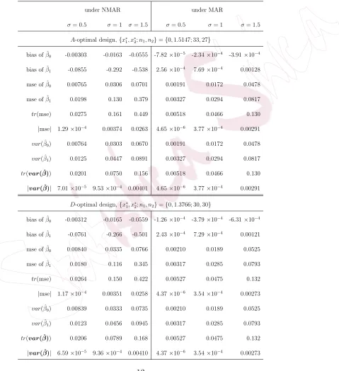
Table 1 presents the performance of the two optimal designs under

dif-ferent missing data mechanisms and difdif-ferent values of σ2_{. The outputs}

under NMAR correspond to the situations where i in (4) has the

corre-spondingσ2 whereas those under MAR correspond to the situations where

i in (4) hasσ2 = 0. In all cases, the responses were simulated with the

cor-responding values of σ2_{. We see that the bias and the mean squared error}

increase as σ2 _{increases. Comparing the two scenarios for the sameσ}2_{, the}

estimates obtained in the presence of a NMAR mechanism have more bias

and larger mean squared errors than those obtained in the presence of the

MAR mechanism. We also find a similar profile for the determinant and

trace of the covariance and the mean squared error matrix.

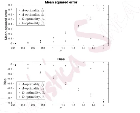
Focusing on the bias and the mean squared error of the estimates in the

presence of a NMAR mechanism, in Figure 1 we plot how this varies with

different values ofσ2 _{under theD- andA- optimal designs found above. The}

mean squared error of each estimate increases with the values ofσ2 _{and the}

estimates are biased downward when σ2 is large. Thus σ2 plays a role in

affecting the performance of any design under NMAR. In the next section

we investigate how we can take account of the effect of σ2 in constructing

Table 1: Simulation outputs ofA- andD-optimal designs across 100,000 simulated data

sets under different missing data mechanisms.

under NMAR under MAR

σ= 0.5 σ= 1 σ= 1.5 σ= 0.5 σ= 1 σ= 1.5

A-optimal design,{x∗

1, x∗2;n1, n2}={0,1.5147; 33,27}

bias of ˆβ0 -0.00303 -0.0163 -0.0555 -7.82×10−5 -2.34×10−4 -3.91×10−4

bias of ˆβ1 -0.0855 -0.292 -0.538 2.56×10−4 7.69×10−4 0.00128

mse of ˆβ0 0.00765 0.0306 0.0701 0.00191 0.0172 0.0478

mse of ˆβ1 0.0198 0.130 0.379 0.00327 0.0294 0.0817

tr(mse) 0.0275 0.161 0.449 0.00518 0.0466 0.130

|mse| 1.29×10−4 _{0.00374 0.0263 4.65×10}−6 _3.77×10−4 _0.00291

var( ˆβ0) 0.00764 0.0303 0.0670 0.00191 0.0172 0.0478

var( ˆβ1) 0.0125 0.0447 0.0891 0.00327 0.0294 0.0817

tr(var( ˆβ)) 0.0201 0.0750 0.156 0.00518 0.0466 0.130

|var( ˆβ)| 7.01×10−5 _9.53×10−4 _{0.00401 4.65×10}−6 _3.77×10−4 _0.00291

D-optimal design,{x∗ 1, x

∗

2;n1, n2}={0,1.3766; 30,30}

bias of ˆβ0 -0.00312 -0.0165 -0.0559 -1.26×10−4 -3.79×10−4 -6.31×10−4

bias of ˆβ1 -0.0761 -0.266 -0.501 2.43×10−4 7.29×10−4 0.00121

mse of ˆβ0 0.00840 0.0335 0.0766 0.00210 0.0189 0.0525

mse of ˆβ1 0.0180 0.116 0.345 0.00317 0.0285 0.0793

tr(mse) 0.0264 0.150 0.422 0.00527 0.0475 0.132

|mse| 1.17×10−4 _{0.00351 0.0258 4.37×10}−6 _3.54×10−4 _0.00273

var( ˆβ0) 0.00839 0.0333 0.0735 0.00210 0.0189 0.0525

var( ˆβ1) 0.0123 0.0456 0.0945 0.00317 0.0285 0.0793

tr(var( ˆβ)) 0.0206 0.0789 0.168 0.00527 0.0475 0.132

Figure 1: Mean squared error and bias of the estimates that were computed using the

4. Optimal design under NMAR

We first provide intuition behind why new theory needs to be developed

in constructing optimal designs when NMAR is present, then present

de-tails concerning our investigation into approximating the missing indicator

probability, and consider broadening the framework to include bias into the

optimality criterion.

4.1 Incorporating NMAR into the design framework

When missing data are present, we seek to minimise a function of

E{[M(ξ,M)]−1_{} as this can be viewed as a surrogate for minimising the} corresponding function of E[var( ˆβ|M)]. Evaluating this expectation is

not straightforward and must be approximated. Imhof, Song, and Wong

(2002) approximate it by {E[M(ξ,M)]}−1_{, while Lee, Biedermann, and} Mitra (2017) first take a 2nd order Taylor expansion of [M(ξ,M)]−1 _and then take the expectation.

Regardless, both approaches assume MAR, and the expectations involve

taking expectations of the missing data indicators E(mi) = P(xi) that

are then components of the resulting optimality criterion. To account for

NMAR when finding optimal designs, we use P(xi, yi), where P(xi, yi) =

E(mi|xi, yi) is now random.

where the expectation is taken with respect to yi. This expectation is not

typically available in closed form and we investigate ways to approximate

it in Section 4.2.

A key consideration is the potential for bias. When NMAR is present,

estimates are likely to be biased as is evident from the results in Section 3.

Optimal design criteria then must incorporate bias, or some approximation

to it, to find designs with small MSE. This is discussed in more detail in

Section 4.3.

4.2 Evaluating the expectation of P(xi, yi)

To evaluate the expectation ofP(xi, yi) we consider the specific example

of the NMAR mechanism (3) introduced in Section 3. In principle, the

ap-proach would work with any appropriate NMAR missing data mechanism.

We can write

P(xi, yi) =

exp(γ0+γ1xi+yi)

1 +exp(γ0+γ1xi+yi)

= exp(zi) 1 +exp(zi)

(5)

where zi ∼ N(γ0 +β0 + (γ1 +β1)xi, σ2). Thus exp(zi) has a Log-normal

distribution with parameters given by the mean and variance of zi, and

P(xi, yi) = ₁₊exp_exp(z₍i_z)_i) has a logit-normal distribution with parameters given

is not available in closed form, we consider approximating the expected

value ofP(xi, yi).

The simplest approach replaces zi with its expected value in (5),

E[P(xi, yi)]≈

exp[E(zi)]

1 +exp[E(zi)]

. (6)

This is equivalent to the naive approach of finding an optimal design in

Section 3 which assumes MAR, and we see that it does not perform well.

An improved approximation uses the fact that E[exp(zi)] = exp[γ0+

β0+(γ1+β1)xi+σ2/2], and taking a first order Taylor expansion ofP(xi, yi)

as a function of exp(zi) about the mean of exp(zi),

E[P(xi, yi)] ≈

E[exp(zi)]

1 +E[exp(zi)]

= exp[γ0 +β0+ (γ1+β1)xi+σ 2_/2] 1 +exp[γ0+β0+ (γ1+β1)xi +σ2/2]

, (7)

We also consider approximating the expectation of P(xi, yi) using

nu-merical methods. Write P(xi, yi) = ti for simplicity, we use the function

integral inMatlab to evaluate

E

exp(zi)

1 +exp(zi)

=E(ti) =

Z 1

0

ti

1

σ√2π 1 ti(1−ti)

e−

[logit(_ti)−_µi]2

2σ2 dt_i (8)

We conducted simulation studies to empirically evaluate the

perfor-mance of these methods for approximatingE[P(xi, yi)]. We generated data

σ, and computed the estimated mean of this distribution using the

differ-ent approximations. This was repeated many times and estimates from

the different methods were averaged over the replications and compared

to the “true mean” obtained empirically by averaging the sample mean of

observations over the replications. This process was then repeated for a

range of different values of µ and σ. Our simulation studies showed that

approximations from (6) and (7) performed poorly compared to (8). The

approximation given by (8) gives us very small magnitude absolute

differ-ences for −30≤ µi

σ ≤ 30. We also considered approximating the expected

value using a second order Taylor expansion about exp(zi) as well as first

and second order Taylor expansions aboutzi. We tried using the median of

the logit normal distribution implied by P(xi, yi), available in closed form,

as a surrogate for the expected value. None of them performed as well

as the numerical approximation considered, and we use (8) in our design

framework going forward.

4.3 Incorporating bias into the design criterion

When responses are not missing at random, estimates will be biased.

Hence, instead of simply considering var( ˆβ), we consider broadening the

framework to incorporate bias. We focus on optimising a function of the

coef-ficient estimates β, the mean squared error incorporates both variance andˆ

bias,

m.s.e. ( ˆβ)=E[( ˆβ−β)( ˆβ−β)T]=var ( ˆβ)+hE( ˆβ)−βi hE( ˆβ)−βi

T

.

(9)

We denote E( ˆβ)−β by ∆(σ, ξ), assuming the bias depends on σ as well

as the design. Other more complex bias functions that depend on more

parameters could be considered.

To find optimal designs in the presence of NMAR with good MSE

prop-erties, we numerically approximated the bias function by simulating it over

a range of different pairs of values (σ, ξ). Each simulation step involved

fitting the model and evaluating the bias for the given pair. We then fit

a smooth function, e.g. a second order response surface or a LOESS

func-tion, to these simulated ‘bias data’, and used this funcfunc-tion, B(σ, ξ) say, as

an approximation to the true bias.

In the next section we evaluate how the approach of finding optimal

designs based on the approximation given in (8) and the inclusion of a

bias term performs in the presence of NMAR, and whether it offers any

improvements over the optimal designs that assume MAR.

5. Simulation study

design we simulated a response variable as

yi = 1 +xi+i, i ∼N(0, σ2)

for a given σ2_{. We then introduced missing values into the observed y}

i,

i= 1, . . . , n, through the logistic model

P(xi, yi) =

exp(γ0+γ1xi+yi)

1 +exp(γ0+γ1xi+yi)

with γ0 = −5.572 and γ1 = 2.191. We fit a simple linear regression model

to the complete case data, obtaining estimates of the coefficients, ( ˆβ0,βˆ1),

and their variances, from the cases for whichyi was observed.

We restricted our optimal designs to the class of designs with two

sup-port points. From Lee, Biedermann, and Mitra (2017), the lower bound

of X, 0, was chosen as one of the support points, x∗₁. To find the second support point, x∗₂, we substituted the approximation to E[P(x∗_i, yi)] given

by (8) with mean −5.572 + 1 + (2.191 + 1)x∗_i and a known value of σ2_{, the} value of x∗₁ and w1 = 1−w2 into the mean squared error given in (9). The expected bias term in (9) was treated as being a function of x∗₂ and σ2_, and was approximated numerically. An optimal design was then found by

minimising a function of this matrix with respect to x∗₂ and w2 in Matlab with the fmincon function.

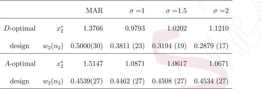
Table 2: The first column from the left shows the optimal designs that assume a MAR

mechanism (6); the other columns show the optimal designs for NMAR mechanisms (5)

with differentσ2_{. In all designs,x}∗

1= 0, n= 60 andw1= 1−w2.

MAR σ=1 σ =1.5 σ =2

D-optimal x∗₂ 1.3766 0.9793 1.0202 1.1210

design w2(n2) 0.5000(30) 0.3811 (23) 0.3194 (19) 0.2879 (17)

A-optimal x∗₂ 1.5147 1.0871 1.0617 1.0671

design w2(n2) 0.4539(27) 0.4462 (27) 0.4508 (27) 0.4534 (27)

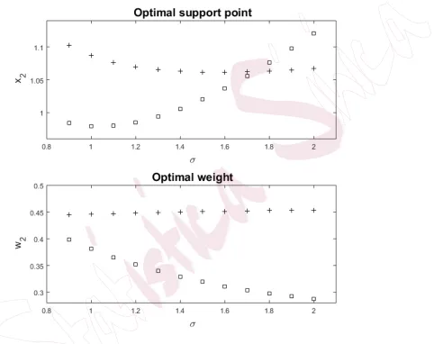
for various different values of σ2, the corresponding weight w2, and the

(rounded) number of replicates,n2, ofx∗2. The optimal designs that account for the impact of NMAR have smallerx∗₂ for both design criteria than those that assume the presence of a MAR mechanism. The optimal weights of

A-optimal designs remain constant in the considered cases whereas w2 of

the D-optimal design decreases with σ2 _{when responses are assumed to be}

NMAR. Figure 2 further illustrates the optimal designs that account for

the impact of NMAR.

To illustrate the performance of these designs we repeatedly simulated

an incomplete data set 200,000 times, using each of the designs given in

Figure 2: “+” correspond to A-optimal designs, “” correspond to D-optimal designs

For each design, we calculated the empirical bias and the mean squared

error for β0 and β1, as well as the determinant and trace of the empirical

mean squared error matrix for (β0, β1). Table 3 presents these results for

various different values of σ.

The designs that assume the presence of MAR have the largest biases

and m.s.e. ( ˆβ) across the board. By taking NMAR into account at the

design stage, we can mitigate some of its effects. For example, theA-optimal

design for σ = 1.5 reduces the bias of ˆβ1 by more than 23% from -0.53864

to -0.41095, and a similar reduction applies to the trace ofm.s.e. ( ˆβ). The

NMAR design with the conjectured value of σ performs best with respect

to the relevant optimality criterion, and the NMAR designs with different

conjectured values of σ also perform well, far better than the designs that

assume MAR.

We consider the problem of assuming the presence of NMAR when in

fact a MAR assumption is reasonable. We evaluated the performance of the

designs given in Table 2 when the missing mechanism was in fact MAR,

with

P(xi) =

exp(γ0+γ1xi)

1 +exp(γ0+γ1xi)

,

where γ0 = −4.572 and γ1 = 3.191. The performance metrics considered

de-Table 3: Performance of various designs in the presence of NMAR mechanism over

200,000 simulated data sets.

σ2_{= 1 in generatingy}

iand in the NMAR mechanism

D-optimal design that assumes A-optimal design that assumes

MAR σ=1 σ=1.5 σ=2 MAR σ=1 σ=1.5 σ=2

bias of ˆβ0 -0.015710 -0.015657 -0.015559 -0.015525 -0.015717 -0.015717 -0.015717 -0.015717

bias of ˆβ1 -0.26664 -0.18472 -0.19344 -0.21511 -0.29240 -0.20739 -0.20208 -0.20313

m.s.e.( ˆβ0) 0.033581 0.027279 0.024665 0.023522 0.030604 0.030604 0.030604 0.030604

m.s.e.( ˆβ1) 0.11689 0.11449 0.12077 0.12403 0.13022 0.10697 0.10728 0.10713

tr(m.s.e.( ˆβ)) 0.15047 0.14176 0.14544 0.14756 0.16083 0.13758 0.13788 0.13774

|m.s.e.( ˆβ)| 0.0035232 0.0025149 0.0025445 0.0026165 0.0037448 0.0026704 0.0026408 0.0026451

σ2_{= 1.5}2_{in generatingy}

iand in the NMAR mechanism

D-optimal design that assumes A-optimal design that assumes

MAR σ=1 σ=1.5 σ=2 MAR σ=1 σ=1.5 σ=2

bias of ˆβ0 -0.054443 -0.054393 -0.054202 -0.054178 -0.054465 -0.054465 -0.054465 -0.054465

bias of ˆβ1 -0.50182 -0.38675 -0.39934 -0.42936 -0.53864 -0.41838 -0.41095 -0.41264

m.s.e.( ˆβ0) 0.076555 0.062639 0.056827 0.054331 0.070012 0.070012 0.070012 0.070012

m.s.e.( ˆβ1) 0.34630 0.32185 0.33703 0.34929 0.37910 0.31198 0.31145 0.31162

tr(m.s.e.( ˆβ)) 0.42285 0.38449 0.39386 0.40362 0.44912 0.38199 0.38146 0.38163

terminant and trace of the empirical mean squared error matrix for (β0, β1).

Table 4 presents these results for MAR optimal designs and different

NMAR optimal designs constructed assuming various values of σ2_{. In this}

simulation, we used a residual variance of σ2 _{= 1.5}2 _{in generating the}

responses under each different design. The empirical biases are negligible,

as expected. We thus focus on the mean squared errors. The designs

generated assuming MAR perform best but there is evidence to suggest

that the loss in assuming a positive value of σ is less severe than the one

incurred when using the MAR design for NMAR data.

6. Case study: Two-group A-optimal design for Alzheimer’s

Dis-ease Trial

As an application, we used data from an Alzheimer’s disease study that

investigated the benefits of administering donepezil, memantine, and the

combination of the two, to patients over a period of 52 weeks, on various

quality of life measures. See Howard et al. (2012) for full details of the

study. We only considered the experimental units in the placebo group

and the donepezil-memantine treatment group that were included in the

primary intention-to-treat sample. The sample size in each group (n1, n2) is

72, resulting in a total sample size of 144. Here we treat the rate of change of

Table 4: Performance of various designs in the presence of a MAR mechanism, i.e.

NMAR with σ2 _{= 0. Responses y}

i are generated with σ2 = 1.52, and over 200,000

simulated data sets.

D-optimal design that assumes

MAR σ=1 σ =1.5 σ=2

bias of ˆβ0 (10−4×) 3.7083 4.0648 5.8203 6.2709 bias of ˆβ1 (10−4×) 4.4560 2.9727 -5.9871 -8.3833

m.s.e. ( ˆβ0) 0.075687 0.061415 0.055479 0.052892

m.s.e. ( ˆβ1) 0.11455 0.19076 0.19898 0.18913

tr(m.s.e. ( ˆβ)) 0.19024 0.25218 0.25446 0.24202

|m.s.e. ( ˆβ)| 0.0056653 0.0078116 0.0081087 0.0077921

A-optimal design that assumes

MAR σ=1 σ =1.5 σ=2

bias of ˆβ0 (10−4×) 3.3924 3.3924 3.3924 3.3924 bias of ˆβ1 (10−4×) 2.4240 2.4140 3.2951 3.3618

m.s.e. ( ˆβ0) 0.068937 0.068937 0.068937 0.068937

m.s.e. ( ˆβ1) 0.11793 0.15299 0.15843 0.15727

tr(m.s.e. ( ˆβ)) 0.18687 0.22192 0.22736 0.22621

cognitive function), as the response variable in a simple linear model,

yi =β0+β1xi+i, i ∼N(0, σ2),

where xi = 0 if subject i is in the placebo group and xi = 1 if subject i is

in the treatment group, i= 1, . . . ,144.

From the data set for the per-protocol analysis, we found 46 patients in

the placebo group and 23 patients in the treatment group who had missing

responses by the end of the study. Assuming that these responses were not

missing at random, a logistic regression model was fit to the missing data

indicator, obtaining

exp(ˆγ0+ ˆγ1xi)

1 +exp(ˆγ0+ ˆγ1xi)

where ˆγ0 = 0.5705 and ˆγ1 =−1.3269. Using the observed responses, we fit a

linear model to the data, obtaining ˆβ0 =−0.10503, ˆβ1 = 0.04302 and σ2 =

0.061432_{. We then used these estimates to construct a NMAR mechanism,}

(5), where the logit-normal variable, ti, had mean γ0+β0 + (γ1 +β1)xi =

0.5705−0.10503−(1.3269−0.04302)xiand varianceσ2 = 0.061432. We used

this information in (6) to approximate the expected NMAR mechanism,

present in the elements of the approximation toE[var( ˆβ|M)] when finding

optimal designs. In practice NMAR is an untestable assumption and there

is no guarantee that such a conjectured mechanism corresponds to the true

Table 5: Fitted coefficients for the approximation functionB(σ, ξ) of ∆(σ, ξ) for ˆβ0(first

row) and ˆβ1 (second row), respectively.

ˆ

λ0 λˆ1 λˆ2 λˆ3 λˆ4 ˆλ5

-2.5282×10−5 _1.8727×10−6 _-1.2511×10−3 _-1.4028×10−8 _8.7490×10−7 _-0.6023

-2.9306×10−5 _-4.1954×10−7 _1.6884×10−3 _2.9213×10−9 _3.1693×10−6 _0.2919

The support points of an optimal design are given as x∗₁ = 0 (placebo) and x∗₂ = 1 (active treatment) since we are comparing two groups. We considered A-optimality with m.s.e. ( ˆβ0) +m.s.e. ( ˆβ1). The optimisation

problem is now in one variable, w2, with the condition w1+w2 = 1.

We conducted simulation studies on designs that hadn2 = 37,38, ...,107

in each design, withσ = 0.04, 0.05, ..., 0.09 in each case, to obtain empirical

biases for ˆβ0 and ˆβ1. Fitting a second order response surface to these

observed biases and values ofn2 andσ, we approximated bias as a function

of n2 and σ, as

B(σ, ξ) = ˆλ0 + ˆλ1n2+ ˆλ2σ+ ˆλ3n22+ ˆλ4n2σ+ ˆλ5σ2

for each estimate ˆβ0 and ˆβ1 (see Table 5).

Using this information, we found the A-optimal design by using the

fmincon numerical method in Matlab. The optimal design resulted in

Table 6: Performance of various designs where n2 is the sample size of the treatment

group andn1= 144−n2for each design.

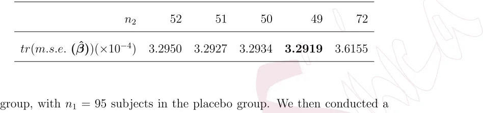
n2 52 51 50 49 72

tr(m.s.e. ( ˆβ))(×10−4_{) 3.2950 3.2927 3.2934 3.2919 3.6155}

group, with n1 = 95 subjects in the placebo group. We then conducted a

simulation study comparing this design with other design candidates using

the estimates ˆβ0, ˆβ1, ˆγ0, ˆγ1 and ˆσ2 in generating responses (both observed

and missing). Table 6 shows the performance of these designs in the

simu-lation. We repeatedly simulated incomplete data under the various designs

and computed the trace of the mean squared error matrix obtained from

each design. The simulation study shows that the A-optimal design that

accounts for NMAR and bias in the experiment performs better than all

other designs considered, and in particular is better than the original

de-sign that assumes equal sample size for both groups. There is about a 9%

(1−3.2919/3.6155)×100% efficiency loss if we use the equal sample size

design instead of the optimal design. This indicates that there is the

poten-tial for obtaining estimates with smaller mean squared error if the proposed

7. Discussion and remarks

There are many open problems left to investigate. A similar

approxi-mation to (7) can be found for nonlinear models with normally distributed

errors, and extensions to generalised linear models are also possible in our

framework.

The designs we find are locally optimal in the sense that they depend

on the unknown model parameters. Our numerical investigations show

that, even when the value of σ2 _{is misspecified at the design stage, the}

designs assuming NMAR with an incorrect σ2 _{perform still better than}

the MAR design when the missing data mechanism is NMAR. For the

other parameters, we assume that good information can be elicited from

the experimenter. If this is not the case, parameter robust design criteria,

such as Bayesian or standardised maximin criteria (see, e.g., Chaloner and

Verdinelli (1995), and Dette (1997)), need to be developed for our approach.

There is a plethora of possible methods to handle the problem of

miss-ing values, in addition to complete case analysis considered here. Other

common approaches include multiple imputation, methods based on the

EM algorithm, Hot Deck methods, and more. We do not investigate these

here, as our approach focuses on the design aspect of the problem, rather

interesting to investigate whether the benefits seen here could be similarly

observed when other methods are used to handle the missing data.

Acknowledgement

The first author’s research was funded by the Institute for Life Sciences

at the University of Southampton. We would like to acknowledge Clive

Holmes; Robert Howard and Patrick Philips for supplying us with the data

from the Domino study RCTN49545035 which was funded by the MRC and

Alzheimer’s Society UK. The second author would like to thank the Isaac

Newton Institute for Mathematical Sciences, Cambridge, for support and

hospitality during the programme Data Linkage and Anonymisation where

work on this paper was undertaken. This work was supported by EPSRC

grant no EP/K032208/1.

References

Ahmad, T., and Gilmour, S. G. (2010). Robustness of subset response

sur-face designs to missing observations. Journal of Statistical Planning

and Inference 140, 92-103.

Chaloner, K. and Verdinelli, I. (1995). Bayesian experimental design: A

review. Statistical Science10, 273-304

optimality criteria. J. Roy. Statist. Soc. Ser. B59, 97-110.

Ghosh, S. (1979). On robustness of designs against incomplete data.

Sankhy¯a: The Indian Journal of Statistics, Series B 204-208.

Hackl, P. (1995). Optimal design for experiments with potentially

fail-ing trials. In Proc. of MODA4: Advances in Model-Oriented Data

Analysis(Edited by C. P. Kitsos and W. G. M¨uller) 117-124. Physica

Verlag, Heidelberg.

Hedayat, A. and John, P. W. M. (1974). Resistant and susceptible BIB

designs. Ann. Statist. 2 1, 148–158.

Herzberg, A. M. and Andrews, D. F. (1976). Some considerations in

the optimal design of experiments in non-optimal situations. J. Roy.

Statist. Soc. Ser. B 38, 284-289.

Howard, R., McShane, R., Lindesay, J., Ritchie, C., Baldwin, A.,

Bar-ber, R., ... and Phillips, P. (2012). Donepezil and memantine for

moderate-to-severe Alzheimer’s disease. New England Journal of Medicine

366, 893-903.

Imhof, L. A and Song, D. and Wong, W. K. (2002). Optimal design of

1145-1155.

Lee, K.M., Biedermann, S. and Mitra, R. (2017). Optimal design for

experiments with possibly incomplete observations. Statistica Sinica.

Little, R. J. A. (1992). Regression with missing X’s: a review. Journal of

the American Statistical Association 87, 1227-1237.

Little, R. J. A. and Rubin, D. B. (2002). Statistical analysis with missing

data (Second Edition). Wiley-Interscience.

Ortega-Azurduy, S. A., Tan, F. E. S. and Berger, M. P. F. (2008). The

effect of dropout on the efficiency of D-optimal designs of linear mixed

models. Statist. Med. 27, 2601-2617.

Pukelsheim, F. and Rieder, S. (1992). Efficient rounding of approximate

designs. Biometrika 79, 763-770.