An alternative method to analyse the biomarker strategy design

DOI: 10.1002/sim.7940

R E S E A R C H A R T I C L E

An alternative method to analyse the biomarker-strategy

design

Cornelia Ursula Kunz

Thomas Jaki

Nigel Stallard

1_{Department of Mathematics and}

Statistics, Lancaster University, Lancaster, UK

2_{Institute of Medical Biometry and}

Informatics, University of Heidelberg, Heidelberg, Germany

3_{Biostatistics & Data Sciences, Boehringer}

Ingelheim Pharma GmbH & Co. KG, Ingelheim am Rhein, Germany

4_{Warwick Medical School, University of}

Warwick, Coventry, UK

Correspondence

Cornelia Ursula Kunz, Boehringer Ingelheim Pharma GmbH & Co. KG. Email: [email protected]

Funding information

National Institute for Health Research, Grant/Award Number:

NIHR-SRF-2015-08-001 ; Medical Research Council, Grant/Award Number: MR/M014525/1 and MR/M005755/1

Recent developments in genomics and proteomics enable the discovery of biomarkers that allow identification of subgroups of patients responding well to a treatment. One currently used clinical trial design incorporating a predictive biomarker is the so-called biomarker strategy design (or marker-based strategy design). Conventionally, the results from this design are analysed by comparing the mean of the biomarker-led arm with the mean of the randomised arm. Sev-eral problems regarding the analysis of the data obtained from this design have been identified in the literature. In this paper, we show how these problems can be resolved if the sample sizes in the subgroups fulfil the specified orthogonality condition. We also propose a different analysis strategy that allows definition of test statistics for the biomarker-by-treatment interaction effect as well as for the classical treatment effect and the biomarker effect. We derive equations for the sample size calculation for the case of perfect and imperfect biomarker assays. We also show that the often used 1:1 randomisation does not necessarily lead to the smallest sample size. In addition, we provide point estimators and con-fidence intervals for the treatment effects in the subgroups. Application of our method is illustrated using a real data example.

K E Y WO R D S

analysis strategy, biomarker, design, interaction, personalised medicine

1

I N T RO D U CT I O N

The focus of modern medicine has shifted from broad spectrum treatments to targeted therapeutics leading to new chal-lenges for the design and analysis of clinical trials. Recent developments in genomics and proteomics enable the discovery of biomarkers that allow identification of subgroups of patients responding well to a treatment. Often, little is known

about this subset of patients until well into large-scale clinical trials.1

The impact of genomic variability is often assessed in a biomarker-based design. The general question when using any of these designs is whether different treatments should be recommended for different subgroups of patients. Establishing clinical relevance of a biomarker test for guiding therapy decisions requires demonstrating that it can classify patients

into distinct subgroups with different recommended managements.2_{Several clinical trial designs using a biomarker to}

identify subgroups of patients likely to respond to a treatment have been proposed in the literature. The most commonly

used designs are the enrichment design and the biomarker stratified design.3,4

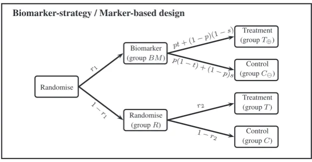
Another currently used design incorporating a predictive biomarker is the so-called biomarker strategy design (or

marker-based strategy design).2,5,6 _{Within this design, patients are randomised either to have their treatment based on}

the biomarker (ie, biomarker-positive patients receive a new treatment while biomarker-negative patients receive the

standard treatment) or to be randomly assigned to treatmentTor control groupC(see Figure 1).

. . . . This is an open access article under the terms of the Creative Commons Attribution License, which permits use, distribution and reproduction in any medium, provided the original work is properly cited.

© 2018 The Authors.Statistics in MedicinePublished by John Wiley & Sons, Ltd.

FIGURE 1 Biomarker-strategy/marker-based design

An alternative variant of the biomarker strategy design would not randomise patients in the randomised arm but treat

everyone in this arm with the control treatment.2,3,7_{Although this design is a special case of the design described above}

(the probability to be randomised into the treatment arm is set to 0), this special case is more frequently used.8_{The main}

criticism here is that a huge proportion of the patients receive the same treatment.9_{Furthermore, given that all patients in}

the randomised arm receive the control treatment, this variant of the biomarker-strategy design cannot establish whether

the new treatment would be beneficial for biomarker-negative patients as they all receive the control treatment.3

Conventionally, the results of a biomarker-strategy design are analysed comparing the biomarker-led arm (armBM)

to the randomised arm (armR) (see Figure 1). The efficiency of this analysis has been investigated.8,10_{However, all}

crit-icisms are focusing on special cases of the biomarker-strategy design: Firstly, they all assume that randomisation to the

biomarker-led and the randomised arm is equal. Secondly, Hoering et al8_{and Young et al}10_{both considered the special}

case of “no randomisation” in the randomised arm, which means that all patients in that arm receive the control treat-ment. Young et al also consider the case of equal randomisation within the randomised arm. While equal randomisation might be frequently used, it is not clear whether this minimises the sample size of the biomarker-strategy design. Fur-thermore, Young et al investigate the efficiency of the design either if there is no treatment effect in the disease-negative patients or if the treatment effect in the disease negative patients is in the same direction as the treatment effect for the positive patients but only half as large.

We hence extend the previous work in the following ways: (1) We investigate the efficiency of the design if the treatment effect in the disease-negative patients is in the opposite direction of the treatment effect for the biomarker-positive patients and (2) we investigate optimal randomisation rules for the design in order to minimise the sample size. Furthermore, we propose a different way to analyse the data obtained from the biomarker-strategy design. The “traditional” analysis

does not exploit all information that can be obtained from the data. Rücker11_{proposed a two-stage randomised clinical}

trial design, which in principle corresponds to the biomarker strategy design with the only difference that patients in the “non-randomised arm” (ie, the biomarker-led arm) choose the treatment they prefer. However, she suggests an analysis

method that allows testing of the overall treatment effect, the self-selection effect and the preference effect. Walter et al12

derive optimal randomisation rules for the abovementioned design by Rücker. Their focus lies only on optimising the first

randomisation while they assume equal allocation to treatment and control in the randomised arm. Turner et al13_{give a}

sample size equation for the design proposed by Rücker. However, like Walter et al, they also assume equal randomisation in the randomised arm. They also assume equal variances across all arms.

The aim of this paper is to adopt the analysis method proposed by Rücker and extend it to the biomarker strategy design by accounting for possible misclassifications using an imperfect assay. We provide equations to calculate the sample size as well as point estimators and confidence intervals for the treatment effects in the biomarker-positive and biomarker-negative subgroups.

2

M OT I VAT I N G E X A M P L E

Brusselle et al14 _{report the results from the AZISAST trial, a multicentre randomised double-blind placebo-controlled}

trial. Patients with exacerbation-prone severe asthma received low-dose azithromycin or placebo as add-on treatment to

the rate of severe exacerbations and the lower respiratory tract infections (LRTI) requiring treatment with antibiotics during the 26-week treatment phase, and one of the secondary endpoints was the forced expiratory volume in 1 second

(FEV1). For the primary endpoint as well as the abovementioned secondary endpoint, no effects were found for the

over-all population. However, opposite effects were found for the primary endpoint for patients with either eosinophilic or

non-eosinophilic severe asthma. For the secondary outcomeFEV1, they report a baseline value of 80.1 (standard

devia-tionSD21.9) for the azithromycin group and a baseline value of 84.8 (20.7) for the placebo group. They also report a mean

difference (between baseline and 26 weeks) of−0.02 for the azithromycin group and a mean difference of−0.90 for the

placebo group. They do not report the values for the two subgroups (eosinophilic or non-eosinophilic severe asthma), so

for our illustrations, we therefore assume the following values:𝜇T+ = 90,𝜇T− = 70,𝜇C+ = 75, and𝜇C− = 95. Patients

with eosinophilic severe asthma are considered “positive.” Furthermore, we assume𝜎T+ =𝜎T− =𝜎C+ =𝜎C− =20. For a

prevalence ofp = 0.5 for eosinophilic asthma, the effect in the treatment group isp𝜇T++ (1−p)𝜇T− =80; for the control

group, the effect isp𝜇C++ (1−p)𝜇C− =85; and the overall treatment effect isp𝜇T++ (1−p)𝜇T−− (p𝜇C++ (1−p)𝜇C−) = −5, which roughly reflects the effects observed in the AZISAST trial.

3

N OTAT I O N

LetNdenote the total sample size (assumed to be fixed),r1denote the fraction of patients randomised to the biomarker-led

arm, and letnBM = Nr1 denote the number of patients in the biomarker-led arm. Furthermore, letnR = N(1 − r1)

denote the number of patients in the randomised arm. Letr2denote the fraction of patients within the randomised arm

that receive the experimental treatment andnT = N(1 − r1)r2 denote the sample size for this arm. Furthermore, let

nC = N(1 − r1)(1 − r2)denote the sample size for the control arm of the randomised arm. We assume that a block

randomisation is used so that the sample sizesnBM,nR,nT, andnCare fixed.

Within the biomarker-led arm, patients have their biomarker assessed. Due to cost, ethical, or administrative reasons,

an imperfect assay is used to determine the true biomarker status. Letpdenote the prevalence of the true biomarker status

and lettandsdenote the sensitivity and specificity of the biomarker assay used. Without loss of generality, we assume that

patients with an observed positive biomarker status receive the experimental treatment while patients with an observed

negative biomarker status receive the control treatment. LetnT_⊕ (nC_⊖) denote the number of patients with an observed

positive (negative) biomarker status. The sample sizes follow binomial distributions withnT_⊕ ∼ Binomial(Nr1,p⊕)and

nC_⊖ ∼Binomial(Nr1,p⊖)withp_⊕ = pt + (1 − p)(1 − s)andp_⊖ = p(1 − t) + (1 − p)s = 1 − p_⊕.

The primary endpoint of interest is denoted with Y and follows a normal distribution with mean 𝜇T+ and

vari-ance 𝜎2

T+ for truly biomarker-positive patients receiving the experimental treatment, mean 𝜇T− and variance 𝜎

2

T−

for truly biomarker-negative patients receiving the experimental treatment, mean 𝜇C+ and variance 𝜎

2

C+ for truly

biomarker-positive patients receiving the control treatment, and mean𝜇C−and variance𝜎

2

C−for truly biomarker-negative

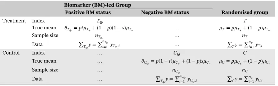
patients receiving the control treatment. Table 1 gives an overview of some of the notation used.

4

T R A D I T I O NA L A NA LY S I S

The traditional analysis of the biomarker-strategy design is to compare the mean of the biomarker-led arm𝜇BMwith the

mean of the randomised arm𝜇_R.15_{The null hypotheses states thatH}TA

0 :𝜇BM = 𝜇Rwhile the alternative hypothesis states

thatH₁TA:𝜇BM ≠ 𝜇R.

TABLE 1 Notation

Biomarker (BM)-led Group

Positive BM status Negative BM status Randomised group

Treatment Index T_⊕ T

True mean 𝜃T_⊕ =pt𝜇T₊+ (1−p)(1−s)𝜇T₋ … 𝜇T=p𝜇T₊+ (1−p)𝜇T₋

Sample size nT⊕ … nT

Data ∑T_⊕𝑦=

∑nT⊕

i=1 𝑦T⊕,i … ∑T𝑦=

∑nT

i=1𝑦T,i

Control Index … C_⊖ C

True mean … 𝜃C_⊖=p(1−t)𝜇C₊+ (1−p)s𝜇C₋ 𝜇C=p𝜇C₊+ (1−p)𝜇C₋

Sample size … nC⊖ nC

Data … ∑T_⊖𝑦=

∑nC⊖

i=1 𝑦C⊖,i ∑C𝑦=

∑nC

LetZBM andZRbe defined asZBM =

∑

T_⊕𝑦+

∑

C_⊖𝑦 Nr1

andZR =

∑

T𝑦+

∑

C𝑦 N(1−r1)

. A test statistic for the hypothesis above is then given by

ZBM−ZR √

̂

VAR[ZBM−ZR]

. (1)

The expected value and variance of the test statistic as well as an estimator for the variance can be found in Appendix A.

4.1

Criticism

Although the biomarker strategy design is sometimes regarded as the gold standard, there is also a lot of criticism regarding the trial design and the analysis of the data. The main problem with the traditional analysis is that it does not distinguish between a situation where there is only an overall treatment effect (but no treatment-by-biomarker interaction effect), a situation where there is only an interaction effect (but no treatment effect), and a situation where there is both a treatment and an interaction effect. This “inability” leads to the following problems:

• Problem 1 “No interaction effect”: As mentioned above, the traditional analysis cannot distinguish between the

treatment and the interaction effect. If there is no interaction effect, we have𝜇T+−𝜇C+ =𝜇T−−𝜇C− =𝜇T•−𝜇C•. In

this case, the expected value of the test statistic for the traditional analysis is E[𝜇BM −𝜇R] = (tp+ (1−p)(1−s) −

r2)(𝜇T• − 𝜇C•). So, as long astp + (1 − p)(1 − s) − r2 ≠ 0 and𝜇T• − 𝜇C• ≠ 0, we observe a difference between

the mean of the biomarker-led arm and the randomised arm even if there is no treatment-by-biomarker interaction effect.

• Problem 2 “Biomarker assay not predictive”:As Freidlin, McShane, and Korn2 _{noted before for a design with}

r2 = 0, it is still possible to observe a difference between the means even if the biomarker assay is not predictive, ie,

t = s = 0.5. In general, ift = s = 0.5, the expected difference between the two arms is(0.5−r2)(p(𝜇T+−𝜇C+) + (1−

p)(𝜇T−−𝜇C−)), which is the same as(0.5 − r2)times the “overall treatment effect.” Hence, we would still observe

a difference between the biomarker-led arm and the control arm (randomised arm) as long as there is an “overall

treatment effect” and 0.5 − r2 ≠ 0. If the observed difference is positive, we would recommend to use the assay to

inform about the treatment a patient should receive although the assay is not predictive.

• Problem 3 “Arbitrary randomisation”: The expected value of the test statistic for the traditional analysis depends on the arbitrary randomisation ratior2since E[𝜇BM−𝜇R] =tp(𝜇T+−𝜇C+) + (1−s)(1−p)(𝜇T−−𝜇C−) −r2(p(𝜇T+−𝜇C+) + (1−p)(𝜇T−−𝜇C−)). It can be shown that ifr2= (pt(𝜇T+−𝜇C+) + (1−p)(1−s)(𝜇T−−𝜇C−))∕(p(𝜇T+−𝜇C+) + (1−p)(𝜇T−−

𝜇C−)), the differences between the two means are always zero (E[𝜇BM − 𝜇R] = 0) irrespective of the values of the

other parameters.

4.2

Orthogonality condition

In the previous section, we have seen that the traditional analysis cannot distinguish between the treatment and the

interaction effect. Under Problem 1, we show that the expected value in case there is no interaction effect is E[𝜇BM−𝜇R] =

(tp + (1 − p)(1 − s) −r2)(𝜇T• −𝜇C•) = (p⊕ − r2)(𝜇T• − 𝜇C•). One way of solving this problem is to setr2 = p_⊕. This

ensures that the traditional analysis is now a test for the interaction effect only and that if there is no interaction effect,

the expected value of the test statistic is indeed 0 (the proof can be found in Appendix A). Hence, settingr2 = pT_⊕ is a

requirement in order to be able to interpret the results of the traditional analysis.

We call this the “orthogonality condition” for the traditional analysis as it is similar to the “orthogonality condition” in

a two-way ANOVA, ie, sample sizes in the different cells have to be proportional (in our case,nT_⊕∕nT=nC_⊖∕nC) in order

to distinguish between the different effects.16_{This will also solve Problem 2 as settingr}

2 = p_⊕leads to E[𝜇BM −𝜇R] =

p(1−p)(s+t−1)(𝜇T+−𝜇C+− (𝜇T−−𝜇C−))so that ift = s = 0.5, E[𝜇BM −𝜇R] = 0. Hence, we do not observe a difference between the means of the biomarker-led arm and the randomised arm if the biomarker assay is of no use at all. We also

solve Problem 3, asr2is now fixed top_⊕.

In general, the expected difference between the mean of the biomarker-led arm and the randomised arm can now only

be zero if (a)p = 0 orp = 1, (b)s+t = 1, or (c)𝜇T+−𝜇C+− (𝜇T−−𝜇C−) =0. Case (a) refers to a situation where there are

situation where there is no treatment-by-biomarker interaction effect. While settingr2top_⊕fixes the problems regarding

the traditional analysis, in practice, the value ofp_⊕is often unknown. Hence, a different method that is robust to the

choice ofr2is preferable. Furthermore, there might be other reasons (ethical or financial) why a different value ofr2might

be chosen.

5

A LT E R NAT I V E A NA LY S I S M ET H O D

In order to overcome the abovementioned disadvantage of the traditional analysis method, we propose a different way to analyse the data obtained from a biomarker-strategy design by defining three test statistics that clearly distinguish between the treatment effect, the (so-called) biomarker effect, and the interaction effect.

5.1

Hypotheses

We define the following three effects: (1) the treatment effect, (2) the biomarker effect, and (3) the interaction effect with corresponding null hypotheses

H₀T∶𝜇T−𝜇C=p𝜇T++ (1−p)𝜇T−− (

p𝜇C++ (1−p)𝜇C− )

=0, (2)

H₀B∶ 𝜇T++𝜇C+

2 −

𝜇T−+𝜇C−

2 =0, (3)

H₀I∶ 𝜇T+−𝜇C+

2 −

𝜇T−−𝜇C−

2 =0. (4)

5.2

Test statistics for the treatment, biomarker, and interaction effect

5.2.1

Test statistic for the treatment effect

The two means𝜇_T and𝜇_Ccan be estimated directly from the design by 1

nT ∑

T𝑦 = ZTRand _nC1 ∑

C𝑦 = ZCR, respectively.

Hence, we can define a test statistic for the treatment effect as follows:

TT =

ZTR−ZCR √

̂

VAR[ZTR−ZCR]

. (5)

The expected value and variance of the test statistic as well as an estimator for the variance are given in Appendix B.

5.2.2

Test statistics for the biomarker and the interaction effect

In the following, we derive test statistics for the biomarker and the interaction effect. Note that the null hypotheses for

the biomarker and the interaction effect depend on the means𝜇T+,𝜇C+,𝜇T−, and𝜇C−, which cannot be estimated directly

from the design. However, it is possible to rewrite the null hypotheses in such a way that only parameters that can be

estimated directly from the data are involved. Let𝜃T_⊕ denote the true mean of the biomarker-led treatment arm, and let

𝜃C_⊖denote the true mean of the biomarker-led control arm (see Table 1). It can be shown that in the case that there is no

biomarker (interaction) effect, the following expressions are true:

HB

0 ∶

𝜇T++𝜇C+

2 −

𝜇T−+𝜇C−

2 =0

⇐⇒H₀B∶𝜃T_⊕−𝜇T(pt+ (1−p)(1−s)) − (𝜃C_⊖−𝜇C(p(1−t) +s(1−p))) =0

(6)

HI₀∶ 𝜇T+−𝜇C+

2 −

𝜇T−−𝜇C−

2 =0

⇐⇒H₀I∶𝜃T_⊕−𝜇T(pt+ (1−p)(1−s)) + (𝜃C_⊖−𝜇C(p(1−t) +s(1−p))) =0.

(7)

Now, letZTandZCbe defined as follows:

ZT = ∑

T_⊕

𝑦−nT⊕

nT ∑

T

𝑦 (8)

ZC= ∑

C_⊖

𝑦−nC⊖

nC ∑

C

It can be shown that the left-hand side of Equations 6 and 7 can be estimated by(ZT−ZC) ∕ (Nr1)and(ZT+ZC) ∕ (Nr1),

respectively. Hence, a test statistic for the biomarker effect is given by

TB=

ZT−ZC √

̂

VAR[ZT−ZC]

(10)

and for the interaction effect by

TI=

ZT+ZC √

̂

VAR[ZT+ZC]

. (11)

The expected values and variances as well as estimators for the variances can be found in Appendix C.

5.3

Multiple testing

In cases where little is known about the new treatment under investigation and/or the biomarker used, it might be desir-able to test more than one hypotheses within the same trial. For example, we might be interested in simultaneously testing

the treatment and the interaction effect. Let COVT,B, COVT,I, and COVB,Idenote the covariances between the test

statis-tics for the treatment and the biomarker effect (T,B), the treatment and the interaction effect (T,I), and the biomarker and the interaction effect (B,I). The expected values of the covariances are given by

COVT,B= −

√

Nr1

(

𝜎2

T(1−r2)(pt+ (1−p)(1−s)) +𝜎

2

Cr2(p(1−t) + (1−p)s) ) √

(1−r1)r2(1−r2) (VAR[ZT] +VAR[ZC] −2COV[ZT,ZC]) (

r2𝜎2

C+ (1−r2)𝜎

2

T

) (12)

COVT,I= −

√

Nr1(𝜎2

T(1−r2)(pt+ (1−p)(1−s)) −𝜎C2r2(p(1−t) + (1−p)s) ) √

(1−r1)r2(1−r2) (VAR[ZT] +VAR[ZC] +2COV[ZT,ZC]) (

r2𝜎2

C+ (1−r2)𝜎

2

T

) (13)

COVB,I=

VAR[ZT] −VAR[ZC]

√

VAR[ZT−ZC]

√

VAR[ZT+ZC]

. (14)

LetTdenote the vector containing the three test statistics for the treatment, biomarker, and interaction effect with

T= (_T

T

TB

TI )

approx.

∼ N(𝜇,Σ)

with

𝜇= (_E

[TT]

E[TB]

E[TI] )

,Σ =

( ₁

COVT,B 1

COVT,I COVB,I 1 )

.

Functions likeqmvnormfrom theR-Packagemvtnormor the Mata functionghk()fromStatacan be used in order to

5.4

Sample size calculation

In the following, we give formulae to approximately calculate the sample sizes to test the different hypotheses given above.

To simplify the notation, let𝜎T,𝜎C,𝜎T_⊕,𝜎T_⊖,A,B, andCbe defined as follows:

𝜎2

T =p (

𝜇2

T++𝜎

2

T+ )

+ (1−p) (

𝜇2

T−+𝜎

2

T− )

−𝜇2_T

𝜎2

C=p (

𝜇2

C++𝜎

2

C+ )

+ (1−p) (

𝜇2

C−+𝜎

2

C− )

−𝜇2_C

𝜎2

T_⊕ =pt (

𝜇2

T++𝜎

2

T+ )

+ (1−p)(1−s) (

𝜇2

T−+𝜎

2

T− )

−𝜃_T2

⊕

𝜎2

C_⊖ =p(1−t) (

𝜇2

C++𝜎

2

C+ )

+ (1−p)s

(

𝜇2

C−+𝜎

2

C− )

−𝜃_C2

⊖

A= 𝜎

2

T_⊕ +𝜎

2

C⊖+p⊕p⊖ (

𝜇2

T+𝜇

2

C )

−2(p_⊖𝜇T𝜃T_⊕+p⊕𝜇C𝜃C_⊖ )

r1 +

(1−r2)p2_⊕𝜎2_T+r2p2_⊖𝜎_C2

(1−r1)r2(1−r2)

B= r1r2p⊕p⊖𝜎

2

C+r1(1−r2)p⊕p⊖𝜎

2

T (1−r1)r2(1−r2)

C= −𝜃T_⊕𝜃C_⊖−p⊕p⊖𝜇T𝜇C+p⊖𝜇C𝜃T_⊕+p⊕𝜇T𝜃C_⊖.

The following equations give the sample sizes required to detect a certain effect for the traditional analysis (NTR), the

treatment effect (NT), the biomarker effect (NB), and the interaction effect (NI) based on a two two-sided test with type I

error𝛼and power 1 − 𝛽:

NTR≈ (

z1−𝛼∕2+z1−𝛽

𝜃T_⊕+𝜃C_⊖− (r2𝜇T+ (1−r2)𝜇C) )2(𝜎2

T_⊕+𝜎

2

C_⊖−2𝜃T⊕𝜃C⊖

r1 +

r2𝜎2

T+ (1−r2)𝜎

2

C

1−r1

)

(15)

NT ≈ (

z1−𝛼∕2+z1−𝛽

𝜇T−𝜇C

)2_(1−r2)𝜎2

T+r2𝜎

2

C

(1−r1)r2(1−r2) (16)

NB≈ (

z1−𝛼∕2+z1−𝛽

𝜃T_⊕−𝜃C_⊖−p⊕𝜇T+p⊖𝜇C )2(

r1A−2C

2r1

)

+ √(

z1−𝛼∕2+z1−𝛽

𝜃T_⊕−𝜃C_⊖−p⊕𝜇T+p⊖𝜇C )4(

r1A−2C

2r1

)2

+ (

z1−𝛼∕2+z1−𝛽

𝜃T_⊕−𝜃C_⊖−p⊕𝜇T+p⊖𝜇C )2

B r2 1

(17)

NI≈ (

z1−𝛼∕2+z1−𝛽

𝜃T_⊕+𝜃C_⊖−p⊕𝜇T−p⊖𝜇C )2(

r1A+2C

2r1

)

+ √(

z1−𝛼∕2+z1−𝛽

𝜃T_⊕+𝜃C_⊖ −p⊕𝜇T−p⊖𝜇C )4(

r1A+2C

2r1

)2

+ (

z1−𝛼∕2+z1−𝛽

𝜃T_⊕+𝜃C_⊖−p⊕𝜇T−p⊖𝜇C )2

B r2 1

(18)

It can be seen that all sample sizes depend on the randomisation ratiosr1andr2. Optimal solutions can be found using

a grid search.

5.5

Point estimators and confidence intervals

The test statistic for the interaction effect does not provide an answer to whether the interaction is quantitative (i.e., the treatment effect for biomarker-positive and biomarker-negative patients points in the same direction but has a different magnitude) or qualitative (i.e., the treatment effects for the two subgroups point in different directions). Hence, we derive

point estimators and confidence intervals for the treatment effects𝜇T+ −𝜇C+ and𝜇T− −𝜇C− for the biomarker-positive

and biomarker-negative patients, respectively. In the following, we assume that the true values of the prevalencep,

the sensitivityt, and the specificitysare known (or can be estimated from a different trial). The treatment effects for

biomarker-positive and biomarker-negative patients can be estimated by

̂𝜇T+− ̂𝜇C+ =

1

Nr1

∑ T_⊕> 𝑦+

1

Nr1

∑

C_⊖𝑦− (1−s)

1

nT ∑

T𝑦−s

1

nC ∑

C𝑦

̂𝜇T−− ̂𝜇C− = −

1

Nr1

∑ T_⊕𝑦+

1

Nr1

∑ C_⊖𝑦−t

1

nT ∑

T𝑦− (1−t)

1

nC ∑

C𝑦

(1−p)(t+s−1) . (20)

Assuming that the estimators approximately follow a normal distribution,(1 − 𝛼)% confidence intervals are given by

[

̂𝜇T+− ̂𝜇C+−z1−𝛼∕2 √

̂

VAR[̂𝜇T+− ̂𝜇C+ ]

, ̂𝜇T+− ̂𝜇C++z1−𝛼∕2 √

̂

VAR[̂𝜇T+− ̂𝜇C+ ]]

(21)

[

̂𝜇T−− ̂𝜇C−−z1−𝛼∕2 √

̂

VAR[̂𝜇T−− ̂𝜇C− ]

, ̂𝜇T−− ̂𝜇C−+z1−𝛼∕2 √

̂

VAR[̂𝜇T−− ̂𝜇C− ]]

(22)

with

̂

VAR[̂𝜇T+− ̂𝜇C+ ]

= 1

(p(t+s−1))2 ⎛ ⎜ ⎜ ⎜ ⎝

Nr1∑_T ⊕𝑦

2₋(∑

T_⊕𝑦 )2

(Nr1)2_(Nr1−1) + Nr1∑_C

⊖𝑦 2₋(∑

C_⊖𝑦 )2

(Nr1)2_(Nr1−1)

+(1−s)

2_s2

T

nT + s

2_s2

C

nC

− 2

(Nr1)2(Nr1−1)

∑ T_⊕𝑦

∑ C_⊖𝑦

) (23)

̂

VAR[̂𝜇T−− ̂𝜇C− ]

= 1

((1−p)(t+s−1))2 ⎛ ⎜ ⎜ ⎜ ⎝ Nr1 ∑ T_⊕𝑦2−

(∑ T_⊕𝑦

)2

(Nr1)2(Nr1−1)

+

Nr1

∑ C_⊖𝑦2−

(∑ C_⊖𝑦

)2

(Nr1)2(Nr1−1)

+t

2_s2

T

nT

+(1−t)

2_s2

C

nC

− 2

(Nr1)2_(Nr1−1)

∑ T_⊕ 𝑦∑ C_⊖ 𝑦 ) . (24)

The derivations can be found in the Supporting Information where we also provide the covariance between the two estimators allowing for the construction of joint confidence regions.

6

R E S U LT S

In order to be able to compare the traditional and the alternative analysis method, we setr2 = p_⊕. As shown in Section

4.2, this will ensure that the traditional analysis method provides a test statistic for the interaction effect only. On the basis of the results for the AZISAST trial (see Section 2), we calculated the sample sizes to test the interaction effect using the

traditional and the alternative analysis method for different values of the prevalencep(from 0 to 1 in steps of 0.01) and

the sensitivitytand specificitys(from 0.5 to 1 in steps of 0.1) for a two-sided type I error of𝛼 = 0.05 and a power of 80%.

In the following, we focus on testing the interaction effect only (instead of testing the treatment, the biomarker, and the

interaction effect simultaneously), so no adjustment for the significance level is made. For the traditional analysis,r2is

set top_⊕(as explained in Section 4.2). In order to find the optimal value forr1, we calculated the sample sizes for values

ofr1from 0 to 1 in steps of 0.01. The randomisation ratior1is then chosen so that the resulting sample size is minimised.

Obviously, choosing smaller increments will yield a more accurate value forr1. For the alternative analysis method, we

used a grid search overr1andr2(from 0 to 1 in steps of 0.01). For each combination ofr1andr2, we calculated the resulting

sample sizes and chose the combination that minimises the sample size for given values ofp,t, ands. In order to verify

the obtained sample sizes, we simulated 10 000 data sets and estimated the resulting type I error and power for different scenarios (see Appendix D).

6.1

Results for the traditional analysis to test the interaction effect

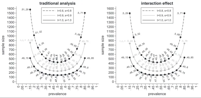
The left-hand side of Figure 2 shows the minimal sample sizes needed for the traditional analysis depending on the

prevalencep, the sensitivityt, and the specificitysfor the AZISAST trial. The black solid line shows the sample sizes for

a perfect biomarker assay, the grey solid line for a biomarker assay witht = s = 0.9, and the black dashed line for a

biomarker assay witht = s = 0.8. The labels show the values for the randomisation ratiosr1andr2with the value ofr1

being the optimal value forr2 = p_⊕.

As expected, we see that the sample size for the perfect assay is smaller than the sample sizes for an imperfect assay with

FIGURE 2 Minimal sample sizes to test the interaction effect using the traditional and alternative analysis method depending on the prevalencep, the sensitivityt, the specificitys, and the randomisation ratiosr1andr2

larger values for the prevalencep. The sample size for the traditional analysis is smallest for a perfect assay, a prevalence

ofp = 0.5, and randomisation ratios ofr1 = 0.47 andr2 = 0.5. In this case, only 142 patients would be needed. If the

prevalence is 0.15, the sample size increases to 516 for the perfect biomarker assay.

For an imperfect assay witht = s = 0.9, the sample size is 231 for a prevalence of 0.5, and hence, in comparison to

a perfect assay, we already need nearly 90 patients more. For a prevalence of 0.15, the sample size increases to 853, and therefore, nearly 340 more patients are needed in comparison with the perfect assay. The sample sizes are even larger

when the sensitivity and specificity are 0.8. In this case, 423 patients are needed ifp = 0.5 and 1580 ifp = 0.15. Compared

with the case of a perfect assay, the sample sizes approximately triple.

In general, it should be noted that the optimal value forr1 is not necessarily 0.5 but varies between 0.47 and 0.51.

However, for a prevalence between 0.05 and 0.95, the difference in sample sizes for the optimal value ofr1andr1 = 0.5

is less than one patient. Therefore, in most cases,r1can be set to 0.5 without a noticeable change in the sample size.

6.2

Results for the alternative method to test the interaction effect

In the following, we show the results for the sample sizes for testing the interaction effect based on our proposed analysis method. The right-hand side of Figure 2 shows the resulting sample sizes for the interaction effect. As before, the black

solid line shows the sample sizes for the perfect biomarker assay, the grey solid line for an assay witht = s = 0.9, and

the black dashed line for an assay witht = s = 0.8. Labels show the optimal values forr1andr2so that the sample size

is minimised for given values ofp,t, ands.

Again, we see that the sample sizes are smaller for prevalences around 0.5 and increase towards smaller and larger values. For example, for a perfect assay and a prevalence of 0.5, the minimal sample size for the interaction effect is 142. It increases to 250 if the prevalence is 0.25 and to 530 if the prevalence is only 0.15. We also see that (as expected) larger

sample sizes are needed if the assay is not perfect. For example, for an imperfect assay witht = s = 0.9, the minimal

sample sizes are 231 (forp = 0.5), 400 (forp = 0.25), and 836 (forp = 0.15). For an imperfect assay witht = s = 0.8,

the following sample sizes result 422 (forp = 0.5), 722 (forp = 0.25), and 1498 (forp = 0.15).

As for the traditional analysis, we note that the optimal value for the randomisation ratior2 isr2 = p_⊕. However,

while this is a requirement for the traditional analysis in order for the results to be interpretable (see Section 4.2), for the

interaction effect settingr2 top_⊕minimises the sample size but is not necessary in order to interpret the results of the

test statistic.

We also see that the optimal value forr1is not necessarily 0.5 but ranges between 0.47 and 0.5. Again, the differences

between the minimal sample size and the one obtained forr1 = 0.5 is less than one patient as long as the second

ran-domisation ratior2 is chosen so that the sample size is minimised givenr1. The situation changes noticeably if both

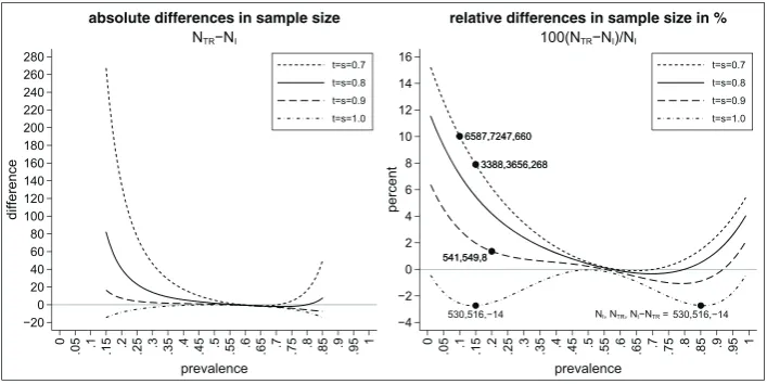
randomisation rules are set to 0.5, which is frequently done. LetN0.5,0.5denote the sample size for the interaction effect

forr1 = r2 = 0.5 and letNmindenote the minimal sample size. Figure 3 shows the absolute difference in the sample sizes

differences vary between 0 and approximately 130 (for a prevalence between 0.15 and 0.85). The absolute difference is even larger for smaller (and higher) values of the prevalence. While we see that the absolute difference of the sample sizes does not depend on the sensitivity and specificity of the biomarker, we see that the relative difference does (see right-hand side of Figure 3). The highest relative differences occur for the perfect biomarker assay (as this has the smallest minimal sample size). Figure 4 shows the absolute differences in sample size for the traditional analysis and the alternative analy-sis for the interaction effect (left-hand side) as well as the relative differences in sample size in percent (right-hand side) . As we can see, the sample size for the traditional analysis is often higher than the sample size for the interaction effect (except for a perfect biomarker assay where the sample size for the traditional design is always lower than the sample size

for the interaction effect). The absolute difference in the sample size might be substantial: for example, fort = s = 0.7

andp = 0.15, the absolute difference in sample size is 268. The relative increase in the sample size is about 8% (from

NI = 3388 toNTR = 3656). We can also see that in cases where the sample size for the traditional analysis is smaller

than the sample size for the interaction effect, the increase in sample size is less than 3%. For example, fort = s = 1 and

p = 0.15, the sample size increases fromNTR = 516 toNI = 530.

FIGURE 3 Difference in sample sizes to test the interaction effect using the alternative analysis method withr1 =r2 = 0.5 or the optimal

randomisation ratios depending on the prevalencep, the sensitivityt, the specificitys, and the randomisation ratiosr1andr2

7

CO N C LU S I O N

This paper investigates the performance of the traditional analysis of the biomarker-strategy design. We derive optimal randomisation rules in order to minimise the sample size for the traditional analysis. We also propose a different analysis method for the data obtained from such a design and explore the properties of this method.

The traditional analysis has been criticised many times.2,9,17,18_{The main problem is that the traditional analysis does not}

distinguish between the treatment and the interaction effect. Hence, it is possible to observe no difference between the mean of the biomarker-led arm and the randomised arm even if there is an interaction effect or to observe a difference between the means even if there is no interaction effect. We show that if the sample sizes in the four subgroups of the biomarker-strategy design fulfil the “orthogonality condition” (ie, are proportional to each other), the abovementioned problems can be solved. However, while the “orthogonality condition” ensures that the traditional analysis provides a

test statistic for the interaction effect only, the value ofp_⊕is often not known as it depends on the true values for the

sensitivity, the specificity, and the prevalence. These values are often unknown at the planning stage of a trial.

To overcome the disadvantages of the traditional analysis, we propose a different analysis method based on the work

of Rücker.11_{We define three different effects than can be measured within the biomarker-strategy design: the treatment}

effect, the biomarker effect, and the interaction effect. This ensures that our analysis can clearly distinguish between the treatment effect and the interaction effect, regardless of the randomisation rules used. We derive test statistics and show how the sample sizes for the three effects can be calculated. Optimal randomisation rules are derived in order to minimise the sample sizes. We also provide point estimators and confidence intervals for the treatment effects in the two subgroups. Furthermore, we show that if the “orthogonality condition” is fulfilled, the sample size for the interaction effect (based on the alternative analysis method) is often smaller than the sample size for the traditional analysis. In cases where the sample size for the alternative analysis method is larger than the sample size for the traditional analysis, the difference is less than 3% of the sample size and therefore often negligible. In general, we therefore recommend to use the alternative analysis method instead of the traditional analysis method.

It should be noted that the biomarker-strategy design is less efficient than the biomarker-stratified design. Shih and

Lin19 _{recently published an evaluation of the relative efficiency comparing the variances of the two designs with each}

other. They conclude that the biomarker-strategy design is less efficient than the biomarker-stratified design, which comes as no surprise given that the biomarker-stratified design contains more information. While the qualitative conclusion of Shih and Lin is correct (ie, the biomarker-stratified design is more efficient than the biomarker-strategy design), their

quantitative results are based on settingr2equal to 0.5. As we have shown, this choice will not lead to the most efficient

design (see Section 6.2). Hence, it remains to be seen how much more efficient the biomarker-stratified design is as compared to the biomarker-strategy design if optimal randomisation rules are used.

AC K N OW L E D G E M E N T S

The authors gratefully acknowledge the valuable input of the associate editor and the reviewer that improved the content and presentation of the paper. The views expressed in this publication are those of the authors and not necessarily those of the NHS, the National Institute for Health Research or the Department of Health or Boehringer Ingelheim Pharma GmbH & Co. KG.

CO N F L I CT O F I N T E R E ST

The authors declare no potential conflict of interests.

O RC I D

Cornelia Ursula Kunz http://orcid.org/0000-0002-8900-9401

R E F E R E N C E S

1. Simon R. Drug-diagnostics co-development in oncology.Front Oncol. 2013;3. Article 315.

3. Sargent DJ, Conley BA, Allegra C, Collette L. Clinical trial design for predictive marker validation in cancer treatment trials.J Clin Oncol. 2005;23(9):2020-2027.

4. Simon R. Clinical trials for predictive medicine.Stat Med. 2012;31:3031-3040.

5. Mandrekar SJ, Sargent DJ. Clinical trial design for predictive biomarker validation: theoretical considerations and practical challenges. J Clin Oncol. 2009;27(24):4027-4034.

6. Sargent D, Allegra C. Issues in clinical trial design for tumor marker studies.Semin Oncol. 2002;29(3):222-230.

7. Hayes DF, Trock B, Harris AL. Assessing the clinical impact of prognostic factors: when is “statistically significant” clinically useful? Breast Cancer Res Treat. 1998;52:305-319.

8. Hoering A, LeBlanc M, Crowley JH. Randomized phase III clinical trial designs for targeted agents.Clin Cancer Res. 2008;14(14): 4358-4367.

9. Simon R. Development and validation of biomarker classifiers for treatment selection. J Stat Plann Inference. 2008;138(2): 308-320.

10. Young KY, Laird A, Zhou XH. The efficiency of clinical trial designs for predictive biomarker validation. Clin Trials. 2010;7: 557-566.

11. Rücker G. A two-stage trial design for testing treatment, self-selection and treatment preference effects. Stat Med. 1989;8: 477-485.

12. Walter SD, Turner RM, Macaskill P, McCaffery KJ, Irwig L. Optimal allocation of participants for the estimation of selection, preference and treatment effects in the two-stage randomised trial design.Stat Med. 2012;31:1307-1322.

13. Turner RM, Walter SD, Macaskill P, McCaffery KJ, Irwig L. Sample size and power when designing a randomized trial for the estimation of treatment, selection, and preference effects.Med Decis Making. 2014;6(34):711-719.

14. Brusselle GG, VanderStichele C, Jordens P, et al. Azithromycin for prevention of exacerbations in severe asthma (AZISAST): a multicentre randomised double-blind placebo-controlled trial.Thorax. 2013;68(4):322-329.

15. Mandrekar SJ, Sargent DJ. Clinical trial designs for predictive biomarker validation: one size does not fit all. J Biopharm Stat. 2009;19(3):530-542.

16. Yates F. The principles of orthogonality and confounding in replicated experiments.J Agric Sci. 1933;23(1):108-145.

17. Mandrekar SJ, Sargent DJ. Predictive biomarker validation in practice: lessons from real trials. Clin Trials. 2010;7(5): 567-573.

18. Simon R. Clinical trial designs for evaluating the medical utility of prognostic and predictive biomarkers in oncology.Personalized Med. 2010;7(1):33-47.

19. Shih WJ, Lin Y. Relative efficiency of precision medicine designs for clinical trials with predictive biomarkers.Stat Med. 2018;37: 687-709.

S U P P O RT I N G I N FO R M AT I O N

Additional supporting information may be found online in the Supporting Information section at the end of the article.

How to cite this article: Kunz CU, Jaki T, Stallard N. An alternative method to analyse the biomarker-strategy

design.Statistics in Medicine. 2018;1–16.https://doi.org/10.1002/sim.7940

A P P E N D I XA: T R A D I T I O NA L A NA LY S I S

The expected value and variance of the test statistic for the traditional analysis are given by

E[ZBM−ZR] = (t−r2)p (

𝜇T+−𝜇C+ )

+ (1−s−r2)(1−p)(𝜇T−−𝜇C− )

=tp(𝜇T+−𝜇C+ )

+ (1−s)(1−p)(𝜇T−−𝜇C− )

−r2(p(𝜇T+−𝜇C+ )

+ (1−p)(𝜇T−−𝜇C−

VAR[ZBM−ZR] =

pt

(

𝜇2

T++𝜎

2

T+ )

+ (1−p)(1−s) (

𝜇2

T−+𝜎

2

T− )

−(pt𝜇T++ (1−p)(1−s)𝜇T− )2

Nr1

+

p(1−t) (

𝜇2

C++𝜎

2

C+ )

+ (1−p)s

(

𝜇2

C−+𝜎

2

C− )

−(p(1−t)𝜇C++ (1−p)s𝜇C− )2

Nr1

− 2 (

tp𝜇T++ (1−p)(1−s)𝜇T− ) (

(1−t)p𝜇C++s(1−p)𝜇C− ) Nr1 + [ p ( 𝜇2

T++𝜎

2

T+− (

𝜇2

C++𝜎

2

C+ ))

+ (1−p) (

𝜇2

T−+𝜎

2

T−− (

𝜇2

C−+𝜎

2

C− ))]

r2 N(1−r1)

− [

(p𝜇T++ (1−p)𝜇T−)

2_{− (p𝜇}

C++ (1−p)𝜇C−)

2]_r2 N(1−r1)

+

p

(

𝜇2

C++𝜎

2

C+ )

+ (1−p) (

𝜇2

C−+𝜎

2

C− )

−(p𝜇C++ (1−p)𝜇C− )2

N(1−r1)

.

(A2)

The variance can be estimated by

̂

VAR[ZBM−ZR] =

∑ T_⊕𝑦2−

(∑

T_⊕𝑦

)2 −∑T_⊕𝑦2

Nr1−1

+∑_C

⊖𝑦 2₋

(∑

C_⊖𝑦

)2 −∑C_⊖𝑦2

Nr1−1

−2 ∑

T_⊕𝑦

∑

C_⊖𝑦 Nr1

(Nr1)2

+N(1−r1)r2 ∑

T𝑦2− (∑

T𝑦 )2

(N(1−r1))2

+ N(1−r1)(1−r2) ∑

C𝑦2− (∑

C𝑦 )2

(N(1−r1))2

.

(A3)

In the following, we show that by setting r2 = p_⊕, the traditional analysis method provides a test statistic for the

interaction effect. According to Equation A1, the expected value is given by

E[ZBM−ZR] =tp

(

𝜇T+−𝜇C+ )

+ (1−s)(1−p)(𝜇T−−𝜇C− )

−r2(p(𝜇T+−𝜇C+ )

+ (1−p)(𝜇T−−𝜇C− ))

=(𝜇T+−𝜇C+ )

p(t−r2) −(𝜇T−−𝜇C− )

(1−p) (r2−1+s) r2=p⊕

= (𝜇T+−𝜇C+ )

p(t−pt− (1−p)(1−s)) −(𝜇T−−𝜇C− )

(1−p) (pt+ (1−p)(1−s) −1+s)

=2p(1−p)(t+s−1) (_𝜇T

+−𝜇C+

2 −

𝜇T−−𝜇C− 2

)

.

(A4)

A P P E N D I XB: T R E AT M E N T E F F ECT

The expected value and true variance of the test statistic for the treatment effect are given by

E[ZTR−ZCR] =p (

𝜇T+−𝜇C+ )

+ (1−p)(𝜇T−−𝜇C− )

(B5)

VAR[ZTR−ZCR] =

p

(

𝜇2

T++𝜎

2

T+ )

+ (1−p) (

𝜇2

T−+𝜎

2

T− )

− (p𝜇T++ (1−p)𝜇T−)

2 N(1−r1)r2

+

p

(

𝜇2

C++𝜎

2

C+ )

+ (1−p) (

𝜇2

C−+𝜎

2

C− )

− (p𝜇C++ (1−p)𝜇C−)

2 N(1−r1)(1−r2) .

(B6)

The variance can be estimated by

̂

VAR[ZTR−ZCR] = = ∑

T𝑦2−

1

N(1−r1)r2

(∑ T𝑦

)2

(N(1−r1)r2)(N(1−r1)r2−1)+

∑ C𝑦2−

1

N(1−r1)(1−r2)

(∑ C𝑦

)2

(N(1−r1)(1−r2))(N(1−r1)(1−r2) −1).

A P P E N D I XC: B I O M A R K E R A N D I N T E R ACT I O N E F F ECT

The expected values are given by

E[ZT] =Nr1𝜃T_⊕−Nr1𝜇T(pt+ (1−p)(1−s)) (C8)

E[ZC] =Nr1𝜃C_⊖−Nr1𝜇C(p(1−t) +s(1−p)). (C9)

The true variances are given by

VAR[ZT] =Nr1

(

pt

(

𝜇2

T++𝜎

2

T+ )

+ (1−p)(1−s) (

𝜇2

T−+𝜎

2

T− )

− (pt𝜇T++ (1−p)(1−s)𝜇T−)

2)

+Nr1p+(1−p+)𝜇2_T+ ((Nr1p+)2+Nr1p+(1−p+))

𝜎2

T

N(1−r1)r2

−2(Nr1𝜇T(tp𝜇T++ (1−p)(1−s)𝜇T−)(1−p+) )

(C10)

VAR[ZC] =Nr1

(

p(1−t) (

𝜇2

C++𝜎

2

C+ )

+ (1−p)s

(

𝜇2

C−+𝜎

2

C− )

− (p(1−t)𝜇C++ (1−p)s𝜇C−)

2)

+Nr1p−(1−p−)𝜇_C2+

(

(Nr1p−)2+Nr1p−(1−p−)

) 𝜎2

C

N(1−r1)(1−r2) −2(Nr1𝜇C((1−t)p𝜇C++ (1−p)s𝜇C−)(1−p−)

)

(C11)

and the true covariance by

COV[ZT,ZC] =Nr1

(

−(tp𝜇T++ (1−p)(1−s)𝜇T− ) (

(1−t)p𝜇C++s(1−p)𝜇C− )

−p_⊕p_⊖𝜇T𝜇C +p_⊖𝜇C

(

tp𝜇T++ (1−p)(1−s)𝜇T− )

+p_⊕𝜇T (

(1−t)p𝜇C++s(1−p)𝜇C− ))

. (C12)

The variances and covariances ofZTandZCcan be estimated as follows:

̂

VAR[ZT] = 1

Nr1−1

⎛ ⎜ ⎜ ⎝ Nr1∑ T_⊕

𝑦2₋

( ∑

T_⊕

𝑦

)2

+Nr1nT_⊕ (

nT_⊕−1 ) s2

T

nT

+Nr1nT_⊕ (

1− nT⊕

Nr1 ) ( 1 nT ∑ T 𝑦 )2

−2Nr1

(

1− nT⊕

Nr1 ) (∑ T_⊕ 𝑦 ) ( 1 nT ∑ T

𝑦)⎞⎟_⎟

⎠

(C13)

̂

VAR[ZC] = 1

Nr1−1

⎛ ⎜ ⎜ ⎝ Nr1∑ C_⊖

𝑦2₋

( ∑

C_⊖

𝑦

)2

+Nr1nC_⊖ (

nC_⊖ −1 )s2

C

nC

+Nr1nC_⊖ (

1−nC⊖

Nr1 ) ( 1 nC ∑ C 𝑦 )2

−2Nr1

(

1− nC⊖

Nr1 ) (∑ C_⊖ 𝑦 ) ( 1 nC ∑ C

𝑦)⎞⎟_⎟

⎠

(C14)

̂

COV[ZT,ZC] = 1

Nr1−1

( − ( ∑ T_⊕ 𝑦 ) ( ∑ C_⊖ 𝑦 ) + ( ∑ T_⊕ 𝑦 )

nC_⊖ ( 1 nC ∑ C 𝑦 ) + ( ∑ C_⊖ 𝑦 )

nT_⊕ ( 1 nT ∑ T 𝑦 )

−nT_⊕nC_⊖ ( 1 nT ∑ T 𝑦 ) ( 1 nC ∑ C 𝑦 )) (C15)

A P P E N D I XD: S I M U L AT I O N R E S U LT S FO R T H E T Y P E I E R RO R A N D P OW E R

In order to verify the sample sizes obtained in Section 6, we simulated 10 000 data sets and estimated the resulting type I error and power (Table D1). The power was estimated using the same values as described in Sections 2 and 6. For

the type I error, the means were set to𝜇T+ = 90,𝜇T− = 70,𝜇C− = 75, and𝜇C− = 55 (ie, assuming that there is no

interaction effect).

TABLE D1 Results for the power based on 10 000 simulations for different values ofp,t,s,r1, andr2

Interaction effect Traditional analysis

p t s r1 r2 NI 𝜶 1−𝜷 r1 r2 NTrad 𝜶 1−𝜷

0.15 0.8 0.8 0.50 0.29 1498 0.0499 0.7927 0.51 0.29 1580 0.0520 0.8211 0.15 0.9 0.9 0.50 0.22 836 0.0510 0.7938 0.50 0.22 853 0.0466 0.8083 0.15 1.0 1.0 0.49 0.15 530 0.0475 0.7877 0.49 0.15 516 0.0482 0.7884 0.20 0.8 0.8 0.50 0.32 974 0.0518 0.7995 0.51 0.32 1015 0.0473 0.8147 0.20 0.9 0.9 0.49 0.26 541 0.0467 0.7939 0.50 0.26 549 0.0461 0.7985 0.20 1.0 1.0 0.49 0.20 341 0.0486 0.7964 0.48 0.20 333 0.0462 0.7795 0.25 0.8 0.8 0.49 0.35 722 0.0500 0.7892 0.50 0.35 745 0.0489 0.8065 0.25 0.9 0.9 0.49 0.30 400 0.0489 0.7967 0.49 0.30 404 0.0473 0.7963 0.25 1.0 1.0 0.48 0.25 251 0.0498 0.7943 0.48 0.25 246 0.0490 0.7876 0.30 0.8 0.8 0.49 0.38 584 0.0478 0.7987 0.50 0.38 598 0.0470 0.8086 0.30 0.9 0.9 0.49 0.34 322 0.0451 0.7900 0.49 0.34 325 0.0533 0.7986 0.30 1.0 1.0 0.48 0.30 201 0.0490 0.7925 0.48 0.30 198 0.0500 0.7830 0.35 0.8 0.8 0.49 0.41 503 0.0462 0.7912 0.50 0.41 512 0.0503 0.8029 0.35 0.9 0.9 0.49 0.38 277 0.0480 0.7870 0.49 0.38 278 0.0473 0.7982 0.35 1.0 1.0 0.48 0.35 172 0.0468 0.7757 0.48 0.35 170 0.0473 0.7697 0.40 0.8 0.8 0.49 0.44 455 0.0478 0.7904 0.50 0.44 461 0.0506 0.7994 0.40 0.9 0.9 0.48 0.42 250 0.0497 0.7829 0.49 0.42 251 0.0496 0.7891 0.40 1.0 1.0 0.47 0.40 154 0.0477 0.7882 0.47 0.40 154 0.0500 0.7787 0.45 0.8 0.8 0.49 0.47 430 0.0476 0.7856 0.49 0.47 433 0.0471 0.8060 0.45 0.9 0.9 0.48 0.46 235 0.0479 0.7817 0.49 0.46 236 0.0488 0.7902 0.45 1.0 1.0 0.47 0.45 145 0.0460 0.7799 0.47 0.45 145 0.0445 0.7885 0.50 0.8 0.8 0.49 0.50 422 0.0493 0.7967 0.49 0.50 423 0.0489 0.7974 0.50 0.9 0.9 0.48 0.50 231 0.0485 0.7865 0.48 0.50 231 0.0455 0.7795 0.50 1.0 1.0 0.47 0.50 142 0.0396 0.7636 0.47 0.50 142 0.0436 0.7613 0.55 0.8 0.8 0.49 0.53 430 0.0463 0.7922 0.49 0.53 430 0.0494 0.7858 0.55 0.9 0.9 0.48 0.54 235 0.0449 0.7841 0.48 0.54 235 0.0460 0.7834 0.55 1.0 1.0 0.47 0.55 145 0.0460 0.7809 0.47 0.55 145 0.0447 0.7870 0.60 0.8 0.8 0.49 0.56 455 0.0482 0.7939 0.49 0.56 454 0.0511 0.7959 0.60 0.9 0.9 0.48 0.58 250 0.0484 0.7847 0.48 0.58 249 0.0467 0.7791 0.60 1.0 1.0 0.47 0.60 154 0.0492 0.7966 0.47 0.60 154 0.0471 0.7973 0.65 0.8 0.8 0.49 0.59 503 0.0498 0.7998 0.49 0.59 501 0.0521 0.8003 0.65 0.9 0.9 0.49 0.62 277 0.0459 0.7881 0.49 0.62 275 0.0430 0.7891 0.65 1.0 1.0 0.48 0.65 172 0.0412 0.7645 0.48 0.65 170 0.0390 0.7657 0.70 0.8 0.8 0.49 0.62 584 0.0510 0.7985 0.49 0.62 582 0.0488 0.7921 0.70 0.9 0.9 0.49 0.66 322 0.0465 0.7908 0.49 0.66 320 0.0492 0.7888 0.70 1.0 1.0 0.48 0.70 201 0.0528 0.7974 0.48 0.70 198 0.0452 0.7855 0.75 0.8 0.8 0.49 0.65 722 0.0481 0.7958 0.49 0.65 720 0.0496 0.7915 0.75 0.9 0.9 0.49 0.70 400 0.0496 0.7942 0.49 0.70 396 0.0466 0.7875 0.75 1.0 1.0 0.48 0.75 251 0.0567 0.8028 0.48 0.75 246 0.0524 0.7891 0.80 0.8 0.8 0.50 0.68 974 0.0476 0.8042 0.50 0.68 974 0.0501 0.8010 0.80 0.9 0.9 0.49 0.74 541 0.0453 0.7931 0.49 0.74 536 0.0496 0.7895

TABLE D1 (Continued)

Interaction effect Traditional analysis

p t s r1 r2 NI 𝜶 1−𝜷 r1 r2 NTrad 𝜶 1−𝜷