Delusions in Theoretical Hydrodynamics

(1)

ISSN Online: 2160-0503 ISSN Print: 2160-049X

DOI: 10.4236/wjm.2018.89029 Sep. 29, 2018 387 World Journal of Mechanics

Delusions in Theoretical Hydrodynamics

Alexander Ivanchin

Orpheus Ltd, Tomsk, Russia

Abstract

Theoretical hydrodynamics may lead one into serious delusions. This article is focused on three of them. First, using flowing around a sphere as an exam-ple it is shown that the known potential solutions of the flow-around prob-lems are not unique and there exist nonpotential solutions. A nonpotential solution has been obtained for flowing around a sphere. A general solution of the problem of flowing around an arbitrary surface has been obtained in the quadrature form. To single out a physically realisable solution among a great number of others, it is necessary to add supplementary conditions to the known boundary ones, in particular, to find a solution with the minimum to-tal energy. The hypothesis explaining the reason for sto-talled flows by viscosity is erroneous. When considering a flow-around problem one should use stalled and broken solutions of the continuity equation along with the conti-nuous ones. If the minimum total energy is achieved by the conticonti-nuous solu-tion, it is a continuous flow that will be implemented. If it is achieved by the broken solution, a stalled flow will be realised. Second, the hydrodynamics of a flow is considered exclusively at each point of it. Differential equations are used to describe the flows that are written for a randomly small volume of a flow, i.e., for a point. The integral characteristics of a flow and its inertial properties are neglected in the consideration, which results in the misunders-tanding of the mechanism of the formation of a vortex. The reason for the formation of vortices is related to viscosity, which is a mistake. The formation of vortices is the result of the inhomogeneity of the acceleration field and the inertial properties of a flow. Third, the fictitious values of viscous stresses are used in hydrodynamics. As a matter of fact, viscosity is the momentum diffu-sion and it should be described by the diffudiffu-sion equation included into the Euler system of equations for a viscous fluid. The momentum diffusion leads to the necessity of including the volume momentum sources produced by diffusion into the continuity equation and excluding the viscosity forces from the equation of motion. The problem of a viscous fluid flowing around a thin plate has been solved analytically, the velocity profiles satisfying the experi-ment have been obtained. The superfluidity of helium is not its property. It is How to cite this paper: Ivanchin, A. (2018)

Delusions in Theoretical Hydrodynamics. World Journal of Mechanics, 8, 387-415.

https://doi.org/10.4236/wjm.2018.89029

Received: August 27, 2018 Accepted: September 26, 2018 Published: September 29, 2018

http://creativecommons.org/licenses/by/4.0/

(2)

DOI: 10.4236/wjm.2018.89029 388 World Journal of Mechanics the interaction of helium with a streamlined surface that is responsible for the mechanism of superfluidity. At low temperatures when the quantum proper-ties are most pronounced the momentum transfer from the helium atoms to the streamlined wall becomes impossible, since the value of the energy trans-ferred in the collision of a helium atom with that of the wall is smaller than the permitted quantum of energy. This mechanism takes place in the case of a flow in capillaries. Under a hydrodynamic flow-around superfluidity does not manifest due to the occurrence of stalled flows. The hypothesis of the disap-pearance of the viscous stresses at low temperatures is erroneous. The viscous stresses cannot disappear since they do not exist in nature. The theory of representing superfluidity as a phase transition accompanied by the forma-tion of the combined viscous and nonviscous phases is a mistake.

Keywords

Nonpotential Flow Around, Nonuniqueness of Flow around a Sphere, Flow around Arbitrary Bodies, Eddy Formation, Viscous Flow, Diffusion and Viscosity, Viscous Flow along a Plate

1. Introduction

In theoretical hydrodynamics there exist serious delusions, both mathematical and physical ones, which lead to erroneous conclusions and misunderstanding in the physics of the flow.

The Euler system of the differential equations of the mechanics of fluid consists of the continuity equation, the momentum-conservation equation or the so-called equation of motion, the energy equation and that of thermodynamic relations [1]. At present the continuity equation is the starting one for steady-state flows. When solving it one derives the field of velocities to define the pressure from the equation of motion.

It is considered that if the potential solution of the continuity equation is found, which is thought to be unique without proof, then the problem has been solved. This is a delusion. In addition to the potential solution, the continuity equation has some nonpotential solutions, which leads to a revision of the knowledge about the physics of the flow of fluids. To obtain a physically realizable solution, it is necessary to add supplementary conditions, e.g. the minimum energy condition, to the boundary and initial ones that are used at present. Other variants are also possible.

The second delusion is that only differential characteristics of a flow are taken into account, the conservation laws are written for a point, whereas the integral characteristics, such as the moment of inertia, are ignored. As a result, the mechanism of the formation of vortices is ignored in the consideration.

(3)

DOI: 10.4236/wjm.2018.89029 389 World Journal of Mechanics history of development, encounters insuperable difficulties in the solution of simple problems, e.g. calculation of a flow near the tip of a flat plate. The reason for this is the wrong, in the physical sense, statement of the problem. From the point of view of molecular physics, there are no viscous shear stresses. It is especially evident in the case of a gas.

The non-uniqueness of the solution of the problem of flow about of a contour is considered in Section 2 and obtain its general solution in quadrature form. Section 3 deals with the formation of vortices in stalled flow. In Section 4, viscosity is considered from the position of momentum diffusion.

2. Flowing around a Sphere

The convolution of two functions [2] f x y z1

(

, ,

)

and f x y z2

(

, ,

)

is denoted by

∗

_{and determined in this way}

(

) (

)

1 1 1

1 2 1 1 1 1 2 1 1 1 1 1 1

, ,

, , , , d d d

S

x y z S

f f f x y z f x x y y z z x y z

∈

∗ =

_∫∫

− − −

(1)

The symbol S above the sign of convolution

∗

stands for a set with respect to which integration is performed. Let z Z x y=

( )

, _{be the equation of the surface}

S, then (1) looks like

(

)

(

)

(

)

1 1

1 2 1 1 1 1 1 2 1 1 1 1 1 1

,

, , , , , , d d

S

x y S

f f f x y Z x y f x x y y z Z x y x y

∈

∗ =

_∫∫

− − −

(2)

Continuity equation. The continuity equation for a steady-state flow is written as [1]

( )

I q r

∇ =

(3) Here Iis the vector of the momentum density at a point in the flow,

I=ρV₍₄₎ V is the velocity at this point, ρ_{is the fluid density,} q

( )

r is the power of the momentum density sources, r=

{

x y z, ,

}

is the radius-vector, _r₌ _x2₊_y2₊_z2

is its length. The nabla

, , x y z

∂ ∂ ∂ ∇ = _{∂ ∂ ∂} 

 (5)

is the differential gradient operator. The vector is denoted by the bold type, its modulus by the usual one.

If the medium is noncompressible, ρ=const, then the continuity Equation (3) is written as [1]

( )

r V q_ρ ∇ =

(6) The Equations ((3) and (6)), in fact, coincide, with only the right side differing by the presence of the constant coefficient, which for linear equations is not essential.

(4)

DOI: 10.4236/wjm.2018.89029 390 World Journal of Mechanics dependence between the density ρ_{and the pressure}_p_{for the adiabatic process} is as follows [3]

0 0 k p p ρ ρ   =  

  (7) The enthalpy for the adiabatic process is written as

1 0 0 0 1 1 k k p k p H

k ρ p

−       = __ _ − _ − _ _     (8)

Here

c c

_p

,

_v art the thermal capacities at a constant pressure and a constant volume,

k c c

=

p v.

The Bernoulli potential is

1 1

2 2

0 0

0 0 0

1

2 1 2

k

k k

p p

I k p I

B H

k p p

ρ ρ ρ

−         = + = ₋ _  − +_           (9)

Having derived the momentum by (3) it is possible to define the velocity field from (9).

Equation of motion. The equation of motion of a fluid when no volume forces or viscosity exist is the following [1]

1 j

i i

j i

I

I I p

t ρ x ρ x

∂ ₊ ∂ _{= −} ∂

∂ ∂ ∂ (10)

Summation is made with respect to the recurrent indices from 1 to 3. Otherwise (10) is written as

(

)

2 2 ₁

V V V

2 2

V V _p

ρ

   

∇_ _+ ∇ × × = ∇_ _+ × = − ∇

    Ω (11)

Here the symbol ∇ ×_{stands for the differential rotor operation,} V

= ∇ ×

Ω

₍₁₂₎

is the angular velocity. The value of V

ρΩ× ₍₁₃₎ is the density of the Coriolis force. It is worth noting that the Coriolis force is a force rather than the moment of force, it cannot induce the rotation of a fluid. In the general case, according to (11), the velocity is a nonpotential vector. The pressure is a potential, since the force produced by it is the gradient of the pressure.

For an incompressible fluid (11) is written as

2 V 0 2 V p ρ   ∇_ + _+ × =

  Ω (14) For the potential field V= ∇Ψ_{, where} Ψ is the velocity potential, then

V 0

= ∇ × = ∇ × ∇Ψ ≡

(5)

DOI: 10.4236/wjm.2018.89029 391 World Journal of Mechanics and from (14) it is possible to derive the Bernoulli relation

(

)

2 2

0

2 2

V

ρ

_{p p}

ρ

₋ _{= −} ₋

(16) The lower index 0 denotes the parameters whose value is known at some point of the flow. It should be noted that (16) is true only for the potential fields of the momentum and an incompressible fluid.

There are two ways of mathematical description of the motion of a fluid. In the Langrange method an elementary particle of the mass is taken and the equation of motion is written for it. Its coordinates are varied in time.

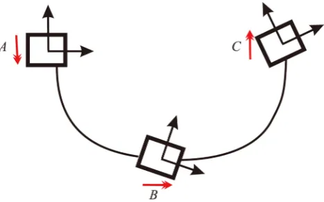
[image:5.595.257.493.359.507.2]

In the Euler method, it is not a material particle that is taken but a fixed volume with a fluid flowing through its surface, and the balance of the forces is considered in this volume. Using the Langrange method it is very simple to show the difference between the potential and nonpotential flow. For the arbitrary element of the mass, according to (12), the angular velocity (15) of its motion in the potential flow is zero, it does not rotate and keeps its orientation even when following a curved trajectory as shown in Figure 1. In the nonpotential flow the angular velocity (12) is not zero and the element of the mass changes its orientation during motion as shown in Figure 2.

Figure 1. Potential flow. The material particles keep their orientation at points A, B, C in spite of the fact that the direction of the motion shown by the red arrows changes by 180˚.

[image:5.595.257.491.547.693.2]

(6)

r

∇ ⋅ =

(18) As shown in [4] this equation has two solutions. The first is the well-known potential one

3 2

r 1

I ,0,0

4πr 4π r

µ µ

= ∇Φ = =

(19) In the present article the Cartesian components are written in the braces. The broken brackets denote that the vector is written in the spherical coordinates with the following sequence of the components: the radial r, the zenith ϑ_{, the}

azimuth ϕ. Substituting ∇Φ from (19) into (18) one derives the Poisson differential equation for the potential Φ:

( )

4π r

µ

_δ

∆Φ =

(20) The solution (20) called a potential is

( )

₄_π ₂ ₂ ₂

4π

r

r _x _y _z

µ µ

Φ = − = −

+ +

(21)

It is the fundamental solution of the Poisson equation.

The vector (19) is the fundamental solution of the Equation (18). The potential vector field produced by the sources q r

( )

will be the convolution of (19)

( )

3

r

r I r

4π

i i

q q

r

µ

∗ = ∗

(22) The convolution of (22) is performed component by component.

The flow of the vector I through a closed sphere with the center at the origin of coordinates is

2 π

2

0 0

d I rr sin d

ϕ

ϑ ϕ µ

=

∫ ∫

(23) It does not depend on the radius of the integration sphere.

As shown in [4], the solution (19) is not unique. There is a vector called neutron

2 2 2

2 3 2

2 r

N 1 3cos 2 ,0,0

2 z x y

r r r

ξ

− −

ϑ

= = +

(24) such that the vector

2 2 2

3 2 3 2 2

r 2 r

I N 1,0,0 1 3cos 2 ,0,0

4π 4π 2

z x y

r r r r r

µ _ξ − − µ ξ _ϑ

+ = + = + +

(7)

DOI: 10.4236/wjm.2018.89029 393 World Journal of Mechanics is the solution of (18), which is checked by the substitution of (25) into (18). Here ξ_{is an arbitrary number, by the terminology}_[4]_{—a neutron charge. The}

vector (25) is nonpotential. The flow N through the sphere with the centre at the origin of the coordinates is

2 π

2

0 0

d N rr sin d 0

ϕ

ϑ ϕ

=

∫ ∫

(26) The addition of N to I does not affect the flow value. At

r

→ ∞

both solutions (19), (24) decrease as ₁_r2_.

The vector (25) is the fundamental solution of nonpotential flows. For the sources q r

( )

the field of velocities produced by them will be the convolution

( ) (

r I N

)

i

q ∗ + ₍₂₇₎

similar to (22).

Delta-function. The general form of the δ-function is [2]

( )

0 n

n

δ ∞δ

=

∑

(28) Here

δ

( )n is the derivative of order n of the δ-function, it is presented as

( )

, ,

x y z

x y z x y z

x y z

m m m n n

n

m m m m m m

m m m x y z

δ δ = + + =λ ∂

∂ ∂ ∂

∑

(29) Here

λ

m m mx y z are the arbitrary constants, the nth derivative of the δ-function

is the linear combination of all its mixed derivatives of the order n.

The presentation of the δ-function in the form (28) should be taken into account in the solution of the Equation (18). A complete solution is obtained by the addition of the linear combination of all derivatives of (25) to the solution (25). The vector (25) tends to zero as ₁_r2_at

_r

_{→ ∞}

_{, its first derivative as}

3

1r and so on.

The derivative δ-function of order n is a multipole of order n. Inclusion into the consideration of the nth derivatives in (28) means the addition of the multipoles of the nth order to the solution (25).

The potential source dipole. The homogeneous flow with a constant momentum density oriented parallel to the z-axis and directed from

+∞

to

−∞

_{is written as}

{

}

w= − 0,0,w = −wcos , sin ,0

ϑ

w

ϑ

(30) The field of the dipole source with the z-axis as the axis of symmetry is obtained by differentiating (19) with respect to z and the replacement of µ_by the dipole moment µ

{

2 2 2

}

5 3

I

I 3 ,3 ,2 2cos ,sin ,0

4π xz yz z x y 4π

z r r

µ

_ϑ

∂

= = − − =

∂

 



(31) The dipoles and their moments are designated by one upper point and the quadrupoles by two points.

(8)

DOI: 10.4236/wjm.2018.89029 394 World Journal of Mechanics r R= _{one derives the known relation}_[1]

3 2πwR

µ

=

₍₃₂₎

As a result one obtains the potential velocity field in flowing around a sphere

3 3

w I 1 cos , 1 sin , 0

2

R R

w

r ϑ r ϑ

    + =  −   +       (33)

The neutron vector dipole. The neutron vector dipole (24) with the z-axis as the axis of symmetry is written in the spherical coordinates as

(

)

3 N

N 8cos 3cos 2 1 , sin 3sin 3 , 0

z r

ξ _ϑ _ϑ _ϑ _ϑ

∂ = = − − − ∂   (34) The quadrupole potential source. Differentiating with respect to z (31) one derives the potential component quadrupole in the form

(

) (

)

{

2 2 2 2 2 2 2

}

2 2

7

4 3

I 4 , 4 , 3 3 2

4π

1 3cos 2 , 2sin 2 , 0

x x y z y x y z z x y z

r

µ

µ _ϑ _ϑ

= − + − + − + − = +    (35)

Here µ is the source quadrupole moment. The vector flow (35) through a sphere is

2 π

2

0 0

d I rr sin d 0

ϕ

ϑ ϕ

=

∫ ∫



(36) The sum of the radial components (24) and (35) on the sphere is

2 2

2 1 3cos 2 ₀ 2 r r N I R R µ ϑ ξ +   + =_ + _ =     (37) at 2 2 R µ _ξ = −  (38) which taking into account (26) and (36) means that the vector

(

)

1 w I+ + λ N I+

(39) is the solution of the continuity Equation (18) at the arbitrary parameter λ1, i.e.

the known solution of the problem of flowing around a sphere (33) is not unique. The field (39) decreases at infinity as ₁_r2_{due to the neutron component (24),}

whereas the potential field (31) decreases as ₁_r3_.

The energetics of the flow around a sphere. The value of

(

)

1 I+λ N I+

 

(40) is the inherent field of a streamlined sphere. The kinetic energy of the field momentum (40) K is

1 2 3

K K= +K +K

₍₄₁₎

(9)

( )

2 2

1 I I d π₄

V

K =

_∫∫∫

 ⋅ V = Rw

(42)

(

) (

)

(

)

2

2 1 7

148π N I N I d

105 V

K V

R

µ

λ

=

_∫∫∫

+ ⋅ + = 

(43) Integration is performed with respect to the external part of the surface of the sphere. The values of K1 and K2 are the self-energies of the potential and the

neutron components, respectively. The value of µ is arbitrary.

(

)

(

)

3 2 1 I N I d 0

V

K = λ

_∫∫∫

⋅ + V =

(44)

is the interaction energy of the potential and the neutron components.

The potential energy should be added to the kinetic energy (41) to get the total energy. The pressure p acts as the potential energy density for an incompressible fluid, whereas enthalpy for a compressible one. The pressure p can be derived from the equation of motion (14), substituting there the velocity (40) one obtains a complex differential equation. There is no point in solving it, since it is impossible to produce continuous flowing around a sphere.

2.2. Solution of the Problem of Flowing through the Sources on

the Surface

Let us illustrate the solution of the problem of flowing using the example of flowing around a sphere with the radius R with the centre at the origin of the coordinates

2 2 2

z= R −x −y

₍₄₅₎

The modulus of the normal of the external flow to its surface, according to (30), is

cos n

w =w ϑ₍₄₆₎

Let a sphere be the source of the density of the momentum having only the radial component which at r→ −R 0_{is equal to}w_n, and at r→ +R 0_is equal to −wn. In passing through the surface of the sphere the momentum density undergoes an abrupt change equal to −2wn. It means that the surface of the sphere S is the carrier of the delta-function of the simple layer [2], and in (3) the function of the source in the spherical coordinates is

( )

r n S

q = −w

δ

₍₄₇₎

In the spherical coordinates only the radial component has the source on the sphere, the direction of the normal to the surface coincides with the coordinate line, therefore, the source (47) is a scalar. In the general case of an arbitrary surface it will be a vector. The flow of the vector wn through the area element dS will be wcos d

ϑ

S_{, its contribution to the potential at the point r will be}

2

1 1 1 1 1

1 1 1 1

2 2 2

1

cos _d cos sin _{d d} cos sin _{d d}

r r ₂ _{1 2}

wR wR

w S

r rR R

ϑ ϑ ϑ _{ϑ ϕ} ϑ ϑ _{ϑ ϕ}

γ γ

= =

− ₋ ₊ ₋ ₊



(10)

DOI: 10.4236/wjm.2018.89029 396 World Journal of Mechanics The lower index 1 means that the given value refers to the sphere S, the radial component of the area element is 2

1 1 1

dS R= sin d d

ϑ ϑ ϕ

. The problem is axially symmetric relative to the z-axis, therefore, it is possible to assume ϕ=0 without a loss of generality. The velocity potential is

( )

2π π

1 1

1 ₂ 1

0 0

2π π

1 1 1 1

0 0 0 2 2 sin cos d d

4π _{1 2}

d sin cos d

4π cos 3 n n n wR wR _P w R r ϑ ϑ

ν ϕ ϑ

γ

ν ϕ ϑ ϑ γ ϑ

ν ϑ

∞

=

Φ = −

− + = − = −

∫ ∫

∑

∫ ∫

    _

(49)

Here it is designated

R r

=



₍₅₀₎

1 1 1

cos cos cos sin sin

γ = ϑ ϑ + ϕ ϑ ϑ₍₅₁₎

ν

is an arbitrary parameter. The expansion in terms of the Legendre polynomials is used

( )

2 ₀ 1 1 2 n n n P γ γ ∞ = =

−  +

∑



(52)

One can show that

( )

π 2π

1 1 1 1

0 0

cos , 1

4π

d sin cos d _0, ₁

3 n n P n

ϑ

γ

ϑ

ϑ ϕ

=  =_≠



∫ ∫

(53) The Legendre polynomial is expressed in this way [5]:

( )

0

( ) (

₍

_{) (}

)

₎

2 0

1 2 2 !

1

! ! 2 !

2 m n n m n n m n m P

m n m n m

γ γ −

= − − = − −

∑

(54) Here n0 is equal to n/2 with even n and to

(

n−1 2

)

in the case of odd n.

Differentiating (49) with respect to r and assuming r R= one derives the value of the normal component on the surface of a sphere

2 _cos 3 n w w R

ν

_ϑ

=

(55) At ν =3 2R the value of the normal component of the flow velocity on the surface of a sphere is equal to (46), i.e. the solution of the problem of flowing around a sphere.

The potential field of velocities is the convolution (19) with a function of a source (47): 3 r S n S w r ν δ − ∗ (56) The field 3 r _w S n S w r ν δ ₋ _∗ ₊  

(11)

DOI: 10.4236/wjm.2018.89029 397 World Journal of Mechanics streamlined body equal to zero.

A complete solution of the problem of the continuous flow around a sphere is written in the form

(

)

(

I 1 I N

)

w

S n S

w

δ

∗ +

λ

+ +

(58) where the vectors I, I, N  are given by the relations (31), (35), (24). The vector

(

N I

)

S n S

wδ ∗ +

(59) on the surface of a sphere will have a zero radial component of the velocity.

If one takes the arbitrary closed surface S as the S in (58), then the function of the source will be a vector value in the form

( )

q r =wn S

δ

₍₆₀₎

and (58) will be written as

(

)

(

1

)

wn S

δ

∗ +S I

λ

I N+ +w

(61) The function (61) is the solution of the Equation (3) and it is a general solution of the problem of flowing by a steady flow around an arbitrary surface S

in the quadrature form and not only around a sphere. According to (28), for a complete solution one should add the multipoles to (61).

To single out a solution that could be physically realisable, it is necessary to add some additional conditions to the boundary ones, e.g. the requirement for the minimum of the total energy of the system. There can be also other conditions.

There is an opinion that the continuous solution of the continuity equation in the problems of flowing when there are no viscous stresses will be a solution that is physically realisable. Broken and stalled flows are ignored in the consideration without explanation. However, stalled flows can have a total energy less than continuous ones, and they are physically realisable. It takes place under flowing round a sphere, and the noncontinuous solution with the formation of vortices is implemented. Nowadays the occurrence of stalled flows is explained by the effect of viscous stresses, which is impossible. Below in section 4 it is shown that viscous stresses do not exist in nature.

3. Inertial Effects

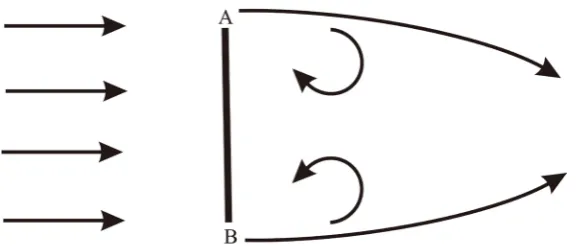
Vortices in a flow occur under stalled flow when a low-density zone is formed behind a streamlined body, which is clearly seen in flowing around an orthogonal plate (Figure 3).

(12)

[image:12.595.231.522.68.191.2]

DOI: 10.4236/wjm.2018.89029 398 World Journal of Mechanics Figure 3. Shown is a thin plate located perpendicular to the running flow. The thickness of its slides at points A and B is much less than the diameter of the vortices occurring behind the plate.

impossible to correlate the formation of vortices with viscosity.

The appearance of the angular velocity (12) is related to the nonpotential character of the flow. However, it changes in the flow from point to point, it is impossible to single out regions rotating as a whole like a solid with the angular velocity similar for all of its points [6]. By the term “vortex” we will understand a fluid domain rotating in such a way that at each point of the domain the angular velocity is approximately the same.

The principal question is which moments of force produce vortices. Pressure cannot produce them in principle, since its force is the pressure gradient, which is a potential value and its work along a closed contour is always zero. If there are no external forces, only the forces produced by the pressure act in a fluid.

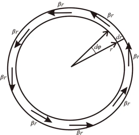
Let us consider a fluid ring in a flow with the radius r and the thickness dr. The element of the ring mass in the cylindrical coordinates is

d d

r r

ρ ϕ ₍₆₂₎

Its moment of inertia is

2π

2 2

0

d d 2π d

r r r r

ρ

ϕ

=

ρ

∫

(63) Let the volume force that in the cylindrical coordinates has only one azimuth component with the density βr₍β _{is the proportionality coefficient) act on a}

fluid (Figure 4). Due to this force, the element of mass (62) is affected by the moment

2_{d d} r r

βρ

ϕ

₍₆₄₎

Integrating this expression with respect to ϕ_{from 0 to}

π

_{, one derives the}

moment of force acting on the ring

2

2π

βρ

r rd

₍₆₅₎

Dividing the moment of force (65) by the moment of inertia (63) one gets that the angular acceleration of the ring is β _{, a constant value. The constants of the}

(13)

[image:13.595.257.489.68.294.2]

DOI: 10.4236/wjm.2018.89029 399 World Journal of Mechanics Figure 4. Shown is the fluid ring, with the volume force of the density βr having only one azimuth component applied to each point on the ring.

Let a flow be formed, due to the differences of the pressure, with the acceleration field

{

}

2

a= γy,0 =γr cos sin , sinϕ ϕ − ϕ

(66) here γ_{is some coefficient of proportionality. In the broken brackets the value} of the vector in the polar coordinates is shown. The acceleration in (66) has a linear dependence on the coordinate. This dependence can be obtained with an arbitrary field of acceleration by means of expansion into the Tailor series near the centre of the domain mass centre

( )

,

( )

0,0 i

( )

0,0 d

i i j

j a

a x y a x

x

∂ = +

∂

(67) The origin of the coordinates is in the centre of the domain mass.

The moment of the force acting on the ring with the inner radius r and the external radius r+dr_{will be derived by the multiplication of the azimuth}

component in (66) by ρr rd _{and the integration with respect to}ϕ from 0 to 2π. As a result, one obtains

2 π

ρ

r rd

− ₍₆₈₎

Comparing (65) and (68) one can see that the acceleration field (66) has the moment of force acting on the ring that ensures spinning of the fluid domain like a solid having the same acceleration at each point.

The rotor ∇ ×a is the angular acceleration. If in a fluid the angular acceleration is a constant value for all the domain points, this domain produces a vortex.

(14)

DOI: 10.4236/wjm.2018.89029 400 World Journal of Mechanics material point has no moment of inertia. The moment of inertia is a characteristic taking into account the inertial properties of a system. The modern theory of hydrodynamics gives them little attention. As a result, the mechanism of the formation of vortices is disregarded. The mathematical description of a flow is made using the system of differential equations, i.e. a flow is considered at each point without integral characteristics. For instance, flowing around a sphere is one of the problems where the stalled character of a flow with the formation of vortices is manifested. All attempts to describe it taking into account viscous stresses are a failure.

4. Momentum Diffusion

At present it is considered that in the flow of a gas or a fluid there exist tangent or the so-called viscous stresses, their value, according to the Newton law is

i ij V

p j

ν ∂

=

∂

(69)

Here

ν

is the viscosity coefficient,

p

ij is the stress tensor and the

nondiagonal components in it are the viscous stresses [1]. The equation of motion (10) has the form

1 ij

i i

j

j j

p V _V V

t x ρ x

∂ ∂ ₊ ∂ ₌

∂ ∂ ∂

(70) The physical reasons for the pressure in a gas and a condensed media are principally different. In the case of a gas, the pressure on the surface is produced only due to the collision of the molecules moving chaotically with the surface. So the source of the pressure in a gas is the kinetic energy of the molecules. The potential energy of the intermolecular interaction does not make contribution to the pressure, since the average distance between the molecules is much larger than the radius of the action of the interatomic forces. This property of a gas is the reason for the implementation of the thermodynamic relations, in particular, the Clapeyron-Mendelyeev law. For the tangential stresses to exist, it is necessary that the molecules be located near the equilibrium position and if they move there would be a force making them return to the previous position.

(15)

DOI: 10.4236/wjm.2018.89029 401 World Journal of Mechanics existence of viscous tangential stresses is erroneous, their inclusion in the equation of motion leads to an incorrect mathematical description of a flow.

In a gas the momentum of a molecule relative to the solid surface can be resolved into the normal and tangential components. In the collision against the wall both components of the molecule can change, since the surface is formed by the atomic sequences. A change of the normal component always leads to a transfer of the surface momentum in one direction—along the normal inside the wall. When the tangential component changes, the molecule has a force effect on the wall in the tangential direction. However, due to the stochastic character of motion, if the average tangential component of the momentum is zero, the gas is immobile, then the average tangential effect on the wall is also zero. When the average tangential momentum projection is not zero and is equal to w, the gas moves along the wall at the velocity w, the reflected molecules transfer to the wall part of the average potential momentum, the wall retards the gas and offers a viscous resistance.

The same happens under a motion inside a gas. If the derivative of the gas velocity in the direction perpendicular to the streamlines is not zero, in the adjacent layers the average velocities of the gas molecules are not the same: the molecules of the layer moving faster penetrate into the slower one and colliding against its molecules transfer an excess momentum. And vice versa, the molecules from the slower layer pass into the faster one retarding it. Thus, the momentum diffusion results in the occurrence of the momentum sources and discharges in the gas volume.

The boundary layer should be considered a diffusion layer, which is described by the equation of diffusion.

A change of the momentum of the elementary volume dQ is caused by two reasons. First, by the effect of the external forces on the volume dQ such as the difference of the pressure. Second, by the addition of the momentum to the volume dQ by diffusion. The total value of the change in the momentum is their sum. The momentum is a vector, one should consider the diffusion blow-in of each of its component through the surface of the elementary volume. Its entry for the time dt is

( )

dJi= ∇ ⋅ ∇

η

I ti d

₍₇₁₎

Here η is the coefficient of the momentum diffusion.

The momentum increment dI is the sum dI dI dJ= 1+ , dI1, we shall call it a

force increment, it is produced by the difference of the pressure p and the external forces. The diffusion momentum dJ changes the momentum of the elementary volume even if there is no difference of the pressure and the external forces. Unlike dI1, it does not enter the Bernoulli Equation (16). This division is

somewhat arbitrary, it serves to illustrate the role of each phenomenon.

(16)

DOI: 10.4236/wjm.2018.89029 402 World Journal of Mechanics contradicts the continuity Equation (3). Therefore, the momentum transferred by the diffusion is divided into two parts

ˆ

dJ dJ dJ= + ₍₇₂₎ here dJˆ is the part of the momentum that passes into the velocity of the particle and part of the dJ, due to the retardation by the environment, passes into the additional pressure

( )

2

d d

2

J p

ρ

=

(73) and this excess pressure affects the motion of the surrounding particles in accordance with the equation of motion (11). Note that here, unlike the force momentum I1, an increase in the velocity can result in an increase in the

pressure. For a number of problems the value of dJˆ is much higher than dJ and it can be neglected in the first approximation dJ.

The diffusion momentum J is derived from the diffusion equation

2 3

, 1

i i

j k j k

J I

t η = x x

∂ ₌ ∂

∂

∑

∂ ∂

(74)

The double summation in this formula is related to the fact that each component of the momentum contributes to the diffusion through all sides of the elementary cube. Besides, in the right side there is the total momentum, whereas in the left one there is the diffusion momentum. This is because the diffusion is produced by the difference in the total momentum, and only the diffusion part of the momentum appears as a result of the diffusion.

For some problems it is possible to separate the force and the diffusion parts, for instance, for the diffusion in a stationary fluid when I1=0, with only the

diffusion part of the momentum remaining. The Equation (74) for this case is written as

2 3

, 1

i i

j k j k

J J

t η = x x

∂ ₌ ∂ ∂

∑

∂ ∂

(75) The diffusion momentum corresponds to the appearance of the volume sources of the momentum with a power equal to the right side (74). These should be added to the continuity Equation (3) and, as a result, one obtains

( )

3 2

, 1

I r i

j k j k I q

x x

η

=

∂ ∇ = +

∂ ∂

∑

(17)

DOI: 10.4236/wjm.2018.89029 403 World Journal of Mechanics first approximation, i.e. the solution of the diffusion equation.

Momentum diffusion near a flat plate. Let us consider a problem in the two-dimensional statement when there is no dependence on the coordinate z

and the vectors have only two components along the abscissa and the ordinate. Let some infinite space be occupied by a stationary fluid, therefore, one can use the diffusion Equation (75). At the origin of the coordinates at the moment

0

t= there occurs an instaneous point source of momentum directed along the axis of abscissa

{ }

{

0

( ) ( ) ( )

}

J= J,0 = Jδ x δ y δ t ,0

(77) and it diffuses into the surrounding space. Here J0 is the power of the

momentum source. Physically the above momentum could be produced in the following way.

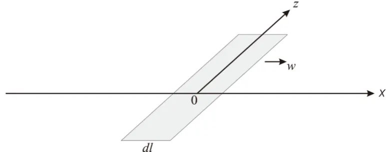
Let in a stationary gas parallel to the axis of abscissa at the origin of the coordinates there be a thin strip of the width dl, which at the moment of time

0

t= moves jumpwise at the distance dx along the abscissa (Figure 5). The gas interacts with the surface of the strip due to the molecule collision. While the strip is immobile, it does not affect the distribution of the molecular velocities. If the strip moves, then due to the collisions of the gas molecules with it, the latter are imparted the momentum, so around the strip there appears a macroscopic motion of the gas diffusing into the surrounding space.

The equation of the momentum diffusion is written as

( ) ( ) ( )

2 2

0

2 2

J J J _J _x _y _t

t η x y δ δ δ

 

∂ ₋ ∂ ₊∂ ₌

 

∂ _∂ ∂ _

(78) If a fluid moves along the abscissa at the velocity

−

w

_{, then the derivative}

with respect to time in (78) should be considered total and then (78) is written as

( ) ( ) ( )

2 2

0

2 2

J _w J J J _J _x _y _t

t x η x y δ δ δ

 

∂ ∂ ∂ ∂

− − _ + _=

∂ ∂ _∂ ∂ _

(79)

For the stationary case ∂ ∂ =J t 0 and the point source constant in time,

( )

t

[image:17.595.152.539.553.705.2]

δ

_{is replaced by unity and (79) changes to}

(18)

( ) ( )

2 2

0

2 2

J J J

w J x y

x η x y δ δ

 

∂ ∂ ∂

+ _ + _= −

∂ _∂ ∂ _ (80)

If a fluid is immobile w=0, then (79) is written as

( ) ( ) ( )

2 2

0

2 2

J J J _J _x _y _t

t η x y δ δ δ

 

∂ ₋ ∂ ₊∂ ₌

 

∂ _∂ ∂ _

(81) Let us introduce the scales of the distance L, the time tm, the momentum

2 0 m

J =J L _{then the variables are brought to the dimensionless form using the}

formulas x L y L t t= χ, = ζ, = mτ,J J= mϒ. Due to the arbitrariness of the scales of L and tm, the following equalities should be fulfilled

2 m L t

η

= ₍₈₂₎

m

w L t= ₍₈₃₎ then the scales are written as

2 m t

w

η

=

(84)

L w

η

=

(85)

2

0 2

m w

J J

η

=

(86) The Equation (79) is written as

( ) ( ) ( )

2 2

δ χ δ ζ δ τ

τ

χ

ζ

∂ϒ ∂ϒ ∂ ϒ ∂ ϒ₋ ₋ ₋ ₌

∂ ∂ ∂ ∂ (87)

Here the property of the δ-function

δ χ

( )

L =

δ χ

( )

L _{is used. No}

parameters enter this equation. The Equation (87) describes the evolution of the dimensionless momentum in the dimensionless coordinates and time.

For estimation let us take the following values of the parameters in (115):

5 2

10 m s,w 1 m s

η

₌ − ₌

. The viscosity coefficient of the air is _{1.5 10 m s}_× −5 2

, then _{10 m,}5 _{10 s}5

m

L₌ − t ₌ − _.

The Equation (87) for a stationary fluid is written as

( ) ( ) ( )

2 2

δ χ δ ζ δ τ

τ

χ

ζ

∂ϒ ∂ ϒ ∂ ϒ₋ ₋ ₌

∂ ∂ ∂

(88)

For the equation in a stationary fluid (81) the velocity w=0, therefore, (83) disappears and the scales L and tm are chosen quite arbitrary. Since further I am planning to turn from a stationary fluid to that moving at the velocity w, the choice of the scales (84) - (86) is the same for the Equation (88).

The stationary Equation (80) for a fluid moving at the velocity equal to unity is presented in the dimensionless variables like

( ) ( )

2 2

δ χ δ ζ

χ

ζ

∂ϒ ∂ ϒ ∂ ϒ₊ ₊ _{= −}

∂ ∂ ∂ (89)

(19)

DOI: 10.4236/wjm.2018.89029 405 World Journal of Mechanics The value J0. The average distance between the molecules λ from the

Clapeyron-Mendelyeev law is written as

1 3 1 3

A

RT kT

pN p

λ=  = 

 

  (90) Here R N k= A is the gas constant, k is the Boltzmann constant, NA is the Avogadro number, T is the absolute temperature, p is the gas pressure. For the air λ is by an order of magnitude larger than the interatomic distance in condensed substances.

The average velocity of the progressive motion of a molecule along the normal to the strip is

kT v

µ =

(91) Here µ_{is the molecule mass. This relation is valid for monoatomic gases.} For polyatomic gases the dependence (91) between the temperature and the progressive velocity at high temperatures is more complicated due to the contribution of the molecule rotations and the intramolecular vibrations. Here the gases are considered for which the relation (91) is fulfilled. The time during which a molecule will cover the length λ_{will be equal to}

1 3 3

2

t

v p kT

λ  µ 

= =  

 

(92) The average length of the free path of the molecules in a gas is much larger than λ_{, it is possible to neglect the colliding ones and consider that half the}

molecules located at the distance λ_{from the strip reach its surface since the}

other half of them move back from it. From the Clapeyron-Mendelyeed equation one derives the number of the moles contained in the volume dV=

λ

dl_per

unit of length along the coordinate z

d _d

p V p _l

RT RT

λ

=

(93) Then the number of the molecules reaching the strip is such

2 3

d 1 _d

2p lλ_RT NA= 2_kTp  l

 

(94) After the collision with the moving strip each molecule will receive from the plate the average momentum αµw directed along the abscissa. The value of

α

_{determines the average value of the transferred tangential momentum in the}

collision of a gas molecule with the atoms of the wall, w is the velocity of the motion of the strip in a jump. Multiplying this value by (94) one derives the momentum transferred from the plate to the gas due to the molecular interaction during the time of the elementary jump t in the form

2 3

0 d

2 w p

J l

kT

αµ

  = _ _

(20)

DOI: 10.4236/wjm.2018.89029 406 World Journal of Mechanics 0

J is the momentum per unit of the length of the plate along the z-axis. Moving source. The continuous motion of the point source of the momentum at the velocity w can be presented in the following way. Let us take the plate length equal to dl w t= d _{. Then (95) will be written as}

2

0 d d

J =w

ω

t=

ηω τ

₍₉₆₎

Here the Equations (84)-(86) are used,

2 3 2 p kT µ ω α= _ _

n

)

2

₎

2

n n

t t x wt y

J x wt y t J

t t t t

θ

η

  − − +   − = − − _ − _ (98)

Summing (98) with respect to n from 0 to N one obtains the solution of the problem on the evolution of the field of the diffusion momentum produced by the moving point source of the momentum in the stationary fluid from time

0 N

t t= < _{to time} t=0_:

(

)

(

)

(

)

(

)

0 2 2 2 0

ˆ , , , ,

1

d exp

4π 4

n N

N n N n

n

n N

N n

n N n N n

J x y t J x wt y t t

x wt y

w

t t t t

ω

_τ

η

= − − = = − = − − = − −  ₋ ₊    = − − _ − _

∑

(99)

With the elementary jump dl→0_{, this sum changes to the integral}

(

)

2 0

(

₍

1

)

2

₎

2

1

1 1

1

ˆ , , exp d

4π t_N 4

x wt y u

J x y t t

t t t t

ω

η

 ₋ ₊  = −  − __ − __

∫

)

=0. If tN< <t 0, then in the sum in (99) summing should be interrupted when tN n− >t and the upper limit in the

(21)

DOI: 10.4236/wjm.2018.89029 407 World Journal of Mechanics upper limit in (100) should be t, and the solution will be written as

(

)

(

)

2 2 2 1 1 1 1

1 exp d

4π _N 4

t

x wt y u

J t

t t t t

ω

η

 ₋ ₊  = −  − _ − _

∫

(101)

Note that as a result of the summation, the momentary character in time of the point source disappears, it becomes constant in time during its movement due to the summation. However, the momentum character of the spatial coordinates remains but changes to the form

δ

(

x wt−

) ( )

δ

y _.

At tN → −∞ (101) changes to

(

)

(

)

2 2 2 1 1 1 1 1

ˆ _exp _d

4π 4

t _{x wt} _y

w

J t

t t t t

ω

η

−∞

η

 ₋ ₊  = −  − __ − __

∫

(102)

Substituting t2= −t t1 in (102) and turning to the moving system of the

coordinates x y, the substitution of x x wt= − one derives

(

)

2 2

2

0 2 2

1 exp d

4π 4

x wt y w J t t t

ω

η

∞  ₊ ₊  = −     

∫

  (103)

In this system of the coordinates the stationary point momentum source is located at the origin of the coordinates, and the fluid moves along the axis of abscissa at the velocity

−

w

. The function (103) is the solution of the stationary equation of diffusion in the moving fluid with the point momentum source at the origin of the coordinates (80).

Using the values (84)-(86) as the scales the solution (103) in the dimensionless form will be presented as

(

)

2 2

0

1 1 exp d

4π 4

χ τ

ζ

τ

∞  ₋ ₊ 

ϒ = − 

 

 

∫

(104)

Here χ=x L ,τ=t t2 m,ζ =y L.

From (104) it follows that the solution does not depend on the time, and the integral is the function of only two dimensionless spatial coordinates χ ζ, . Let us show that (104) is the solution of the stationary equation of diffusion in the moving fluid (89). Substituting the function (104) into (89) one obtains

(

)

2 2

3 0

exp d 0

4

χ τ

ζ

τ

∞_Λ  ₋ ₊ 

− ≡      

∫

(105)

2 2 ₄ 2

χ

ζ

τ τ

Λ = + − − ₍₁₀₆₎

For the Equation (104) to be the solution of the equation (89), it is necessary that (105) be zero at any values of χ ζ, _{. I have failed to analytically prove it,} however, the numerical calculation (105) supports it.

The sign Λ_{determines the sign of the integrand in (105). The equation}

0

Λ = _{has only one positive root}

2 2

* 4 2

(22)

DOI: 10.4236/wjm.2018.89029 408 World Journal of Mechanics At 0< <τ τ*,Λ >0, and at τ τ> *,Λ <0. The integrand in (105) exponentially

tends to zero both at τ→0_and

τ

→ +∞. Really, _Λ_~_τ2_at

_τ

_{→ +∞}_{, and}

the exponent in (105) tends to zero, since its index

→ −∞

at

τ

→ ∞

. At any values of χ ζ, the following equality takes place

(

)

(

)

1 , 2 ,

I

χ ζ

= −I

χ ζ

₍₁₀₈₎

(

)

*

(

)

2 2

1 3

0

, exp d

4

I

χ ζ

τ

χ τ

ζ

τ

 ₋ ₊  Λ

= − 

 

 

∫

(109)

(

)

(

)

*

2 2

2 , 3exp ₄ d

I

τ

χ τ

ζ

χ ζ

τ

∞ _Λ  ₋ ₊ 

= − 

 

 

∫

(110)

As an example, Figure 6 shows the results of the calculation of the integrals

(

)

1 ,

I

χ ζ

and I2

(

χ ζ

,

)

for the abscissa χ=1 and the ordinate ζ within

the interval

( )

0,6 . The curves in the plot are symmetric relative to the axis ζ _,

hence it follows that the equality (108) is fulfilled.

Note that the identity (105) is valid even for a more general form of the functions at the arbitrary ς

(

)

2 2

3 0

exp d 0

4

χ ςτ

ζ

τ

∞_Λ  ₋ ₊ 

− ≡

 

 

∫

(111)

The plate of a finite length. To consider flowing around the plate with a finite length , it is necessary to use the momentum function δ, its carrier is

the segment , i.e. to use the notion of a simple layer. It is determined as [2]

(

,

)

(

( ) ( )

,

)

d

t

f x y f x t y t t

∈

∗ =

_∫



(112) The plate length in the dimensionless form is

[image:22.595.216.540.72.257.2] [image:22.595.211.540.487.687.2]

(23)

L

λ=

(113) The equation (89) is written as

2 2

δ

λ

χ

ζ

∂ϒ ∂ ϒ ∂ ϒ₊ ₊ _{= −}

∂ ∂ ∂ (114)

Here δλ is the δ-function with the carrier the segment λ in the

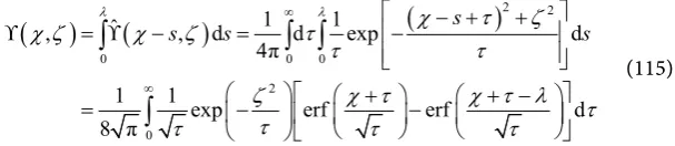
dimensionless variables. Using (104), one derives the solution of the Equation (114) [2]

(

)

(

)

(

)

2 2

0 0 0

2

0

1 1

ˆ

, , d d exp d

4π

1 _{1 exp} _erf _erf _d

8 π

s

s s s

λ λ _χ _τ _ζ

χ ζ χ ζ τ

τ τ

ζ χ τ χ τ λ _τ τ

τ τ τ

∞

 _{− +} ₊ 

ϒ = ϒ − = − 

 

 

    +   + − 

= _− _{ } _ _− _ __

   

 

 

∫

∫ ∫

∫

[image:23.595.235.539.206.272.2]

(115)

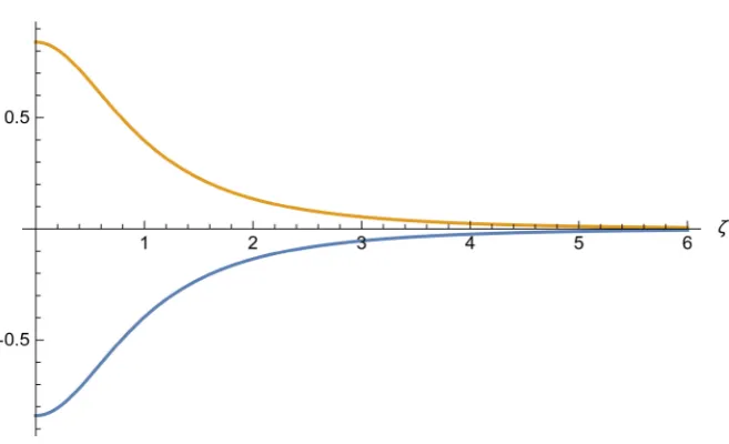
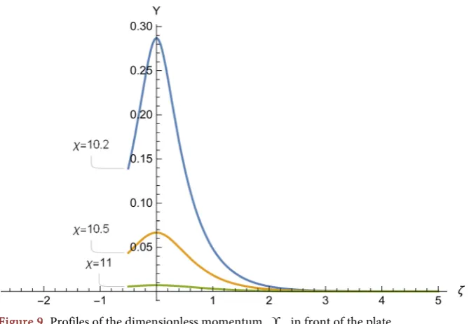
Figures 7-9 show the diffusion momentum ϒ versus the coordinate ζ for the assigned values of χ . The values of χ are shown on the left of the plot, which gives the values of the momentum on the straight lines orthogonal to the plate χ=const_{. In}_{Figure 7}_{these lines go through the plate, in}_{Figure 8}_they cross the axis of abscissa χ behind the plate. In Figure 9 they pass in front of the plate.

The plots are symmetric to the axis of abscissa χ as it follows from (115), therefore, it would be enough to show the plots only for ζ ≥0_{. However, their} behavior on the axis of abscissa at ζ =0 is of interest, therefore, the left half of the profile is shown in the truncated form.

[image:23.595.209.544.431.658.2]

(24)

[image:24.595.208.541.70.289.2]

DOI: 10.4236/wjm.2018.89029 410 World Journal of Mechanics Figure 8. Plots of the momentum ϒ behind the streamlined plate.

Figure 9. Profiles of the dimensionless momentum ϒ in front of the plate.

In Figure 7 one can see that the plot of the momentum on the plate forms an acute angle, i.e. the derivative d dϒ ζ _{on the plate undergoes a break, which}

should be expected, since the plate is the momentum source. Outside the plate the momentum profile has an extremum with the continuous derivative

d dϒ ζ =0_.

In front of the plate there also exists a diffusion momentum shown in Figure 9. However, it disappears quickly with increasing distance from the plate up the flow.

[image:24.595.208.543.310.541.2]

(25)

DOI: 10.4236/wjm.2018.89029 411 World Journal of Mechanics ones. The theory suggested here solves the above problem.

Flow in the cylindrical tube. As it has been shown here, the viscosity coefficient

ν

in (69) is a fictitous value, since there are no shear stresses in gases and fluids. There arises a question how the viscosity coefficient

ν

is related to the coefficient of the momentum diffusion η. One of the main methods of measurement of the viscosity coefficient is the flow in a cylindrical tube [1].

The rate of the flow through a cylindrical tube of the radius R under a laminar flow is [1]

4 4

π π

8 8

R p _{R P}

l

ν ν

∆ =

(116) Here P= ∆p l_{is the difference of pressure per unit of the tube length.}

For the stationary flow of a viscous fluid through a round tube of the radius R

due to the viscosity there is a radial dependence of the velocity u u r=

( )

that is smaller near the tube wall than on the axis. As the boundary condition let us take the adherence condition

( )

0, u r = r R=

(117) The equation of the momentum diffusion for an incompressible fluid in the cylindrical coordinates is written as

u u

u r P

z r r r

η

ρ ∂ − ∂ _ ∂ _=

∂ ∂  ∂  (118)

The velocity u does not depend on z, then ∂ ∂ =u z 0_{and this equation is} brought to the form

u

r P

r r r

η ∂  ∂ 

− _ _=

∂  ∂ 

(119)

The solution of this equation is

2

4ln 5 4

P

u= _ηr +c r c+

(120) Here c4 and c5 are the arbitrary constants, from the limiting condition of

the velocity it follows that c4=0.

The value of the arbitrary constant c5 is determined from the boundary

condition (117).

In a general case, it is necessary to assign the momentum diffusion into the tube wall

r R

u ₌ =

ατ

(26)

DOI: 10.4236/wjm.2018.89029 412 World Journal of Mechanics 2

5 PR₄

c

η

= −

(122) Finally, (120) is presented as

( )

(

2 2

)

4

P u r = _η R −r

(123) which completely coincides with the classical distribution of the velocities across the section of the tube [1]. The flow rate along the tube is determined by integrating (123) with respect to the tube section

( )

2π 4

0 0

π

d d

8

R _R

u r r P

ϕ

η

=

∫ ∫

(124) The relations (116) and (124) coincide, which means that in the experiments on the measurement of the viscosity coefficient it is the coefficient of the momentum diffusion which is determined rather than that of viscosity.

Coefficients of the momentum diffusion and thermal conductivity. The relation of the viscosity coefficient to that of thermal conductivity is called the Prandtl number [1]. The mechanism of the momentum diffusion and the heat transfer is ensured in the same way—by the chaotic motion of the gas molecules and their collision. On the average for a monoatomic gas a kinetic energy of

kT/2 falls at one degree of freedom and 3kT/2 at three degrees of freedom, with the energy, i.e. the heat transferred by all three degrees of freedom. Unlike the heat transfer, the momentum has a definite direction, which is that of the flow of a fluid. The chaotic motion in this direction does not affect the transfer of the momentum that is transferred in the deterministic process. So only two directions remain for the diffusion. Therefore, the Prandtl number for monoatomic gases should be 2/3, which is really observed [7].

Superfluidity of helium. Fluid helium at a temperature below 2.6 K possesses superfluidity [8], i.e. the ability to flow at a large velocity through capillars, which means that the viscosity coefficient is either by orders of magnitude less than the known values or zero.

The diffusion mechanism of viscosity is responsible for superfluidity. At low temperatures the thermal energy of 3kT/2 falling at a helium atom is small and by the laws of quantum mechanics the energy transfer is possible only by quanta. If the energy transferred is less than a quantum, then the momentum cannot be transferred from a streamlined body to helium atoms, which rules out its diffusion, which in turn means that the coefficient of cohesion in (95) α=0_. Superfluidity is not the property of helium nor a phase transition leading to the disappearance of viscous stresses that do not exist in nature. It is the feature of the interaction of helium atoms with the atomic lattice of the surface at low temperatures.