Developing and Evaluating SIMM Forecasting Models

DEVELOPING AND EVALUATING

SIMM FORECASTING MODELS

PRIS, M (MIRAN)

List of essential abbreviations

CCR Counterparty Credit Risk, specific type of risk arising from exposure to a counterparty by means of derivative transactions. CIR Cox-Ingersoll-Ross model for modelling the term structure, based

on short rates.

CSA Credit Support Annex, a legal document that regulates derivative transactions and its credit support (like collateral). It is one of the four elements of an ISDA Master Agreement.

DEV Displaced Exponential-Vašíček, a method for modelling short rates, which is an extension of the Exponential-Vašíček method with the possibility for negative simulated rates.

EaD Exposure at Default, a risk measure used for regulatory capital calculations.

EC Economic Capital, amount of capital that an organization should hold in order to ensure it stays solvent given its risk profile. EV Exponential-Vašíček, a method to model short rates

FRA(t, T, S, τ, N, K) Forward-Rate Agreement with valuation date t, expiry date T, maturity date S, year fraction τ between T and S, notional amount N, and fixed-rate K.

IA Independent Amount. A precursor of IM, which is static (constant) throughout the lifetime of a bilateral netting set.

IM Initial Margin, type of collateral that is bilaterally exchanged, regardless of moneyness of counterparties and segregated. The collateral is supposed to cover 99% of exposure during the MPOR. IMM Internal Model Method, an institution’s specific internal

framework. To be able to use the IMM for collateral calculation, the institution needs to obtain approval from regulators.

(P-/R-)IRS(t, T, τ, N, K) (Payer-/Receiver-) Interest Rate Swap with valuation date t, a vector of payment dates T, tenors τ, notional amount N, and fixed-rate K. The final payment date and maturity date coincide. LIBOR London Interbank Offered Rate

MPOR Margin Period of Risk, the time period between the last margin posting and the unwinding of the counterparty portfolio in case the counterparty defaults. In this thesis the MPOR is assumed 14 calendar days (10 business days).

MTA Minimum Transfer Amount, a threshold that determines at which minimum level (exposure) the collateral should be posted to the other party.

MtM Mark-to-Market, a fair-value measure of an instrument or asset. It is also known as the replacement value of the instrument or asset.

OTC Over-The-Counter

PFE Potential Future Exposure, measure for exposure based on a quantile of the MtM-VM distribution.

RC Regulatory Capital, the amount of capital an organization should hold in order to survive any difficulties, such as market or credit risks.

SA Standardized Approach, a standardized ‘add-ons’-based model for calculating the amount of t0-IM needed for a netting set.

SIMM Standard Initial Margin Model, a standardized sensitivities-based model developed by ISDA for the calculation of t0-IM

VM Variation Margin, a type of collateral that is held only by the in-the-money counterparty in order to reduce exposure.

Contents

1

Introduction

3

1.1

Regulatory reforms

3

1.2

Problem setting

4

1.3

Scope of research

4

1.4

Document Structure

5

2

Bilateral Margining and Regulations

6

2.1

Variation Margin

7

2.2

Initial Margin

8

2.2.1 Calculating Initial Margin at t0 (the regulatory IM) 9

2.2.2 Allowed collateral types 10

3

Challenges for Rabobank

11

3.1

Forecasting future IM

11

4

Modelling Exposure

13

4.1

Potential Future Exposure (PFE)

13

4.2

Margin Period Of Risk (MPOR)

14

4.3

Collateral Modelling

14

4.3.1 Exposure threshold 14

4.3.2 Minimum Transfer Amount (MTA) 14

4.3.3 Collateral balance 15

4.3.4 Obtaining the MtM at non-simulation dates 15

5

Future SIMM forecasting model alternatives

16

5.1

Dynamic SIMM – the benchmark model

16

5.2

Weighted Notional Model

17

5.3

Weighted MtM Model

18

5.4

American Monte Carlo

18

6

Research Setup

21

6.1

Portfolio 1

21

6.2

Portfolio 2

22

6.3

Portfolio 3

23

6.4

Changing the payer-to-receiver swap ratio

24

6.5

Experimental environment

25

6.6

Delta profiles

26

7

Results

31

7.1

Weighted Methods and Dynamic SIMM

31

7.1.1 Weighted MtM versus Weighted Notional 32

7.1.2 Improving the weighted methods 40

7.2

American Monte Carlo and Dynamic SIMM

43

7.3

Impact of volatility

48

7.4

Impact of IM Methods on PFE

48

8

Discussion

54

8.1

Performance and implementation

54

8.2

Getting ready for t

-SIMM

55

10

Future Research

57

11

Bibliography

58

A

t0-IM calculation

60

A.1

Standardized Approach (SA)

60

A.2

SIMM

61

A.2.1 SIMM Calculation Example 62

A.2.2 Concentration risk under SIMM 67

B

Interest Rate Swaps

69

B.1

Characteristics

69

B.2

Valuation

70

B.2.1 Deriving an expression for the forward rate and FRAs 70

B.2.2 Valuing IRS through FRAs 71

C

Term structure modelling

72

C.1

Short-rate models

72

C.1.1 Vašíček Model 72

C.1.2 Exponential-Vašíček (EV) Model 73

C.1.3 Displaced Exponential-Vašíček (DEV) Model 73

Page | 1

Management Summary

Regulations

According to new regulatory requirements, financial market participants (financial institutions and NFC+s) are obliged to exchange collateral margins (Variation Margin and Initial Margin) when trading OTC derivatives. They have two choices to transact such trades (and post corresponding collateral): either by clearing through central clearinghouses (CCPs) and by posting collateral to these central parties or by transacting bilaterally and posting corresponding collateral to each other. Our research focuses on the bilateral margining of OTC transactions.

Variation Margin (VM) is used to cover daily changes of the bilateral netting set’s value (replacement value, marked to market). In essence, when a counterparty is in the money on the bilateral netting set, then that party receives VM. This type of collateral is posted unilaterally. On the other hand, regulators introduce Initial Margin (IM), which is intended to cover the change of netting set value between the last exchange of VM and the unwinding of the bilateral netting set. This type of collateral is needed, because a counterparty may go into default and from that moment on, this defaulting counterparty will not post VM anymore to the non-defaulting counterparty. From that default moment until the unwinding of the netting set (this time period is also called the Margin Period of Risk or MPOR), the non-defaulting party is exposed. Different from VM, IM is posted by both parties to a third party segregated account.

Regulators allow for three ways to calculate IM at t0:

 By using the Standardized Approach (SA), which is an add-on based model.

 By using an initial margin model, developed by one or both counterparties, or by a third party. The requirements for the own-developed model is that the IM should be calculated as a 99% VaR of netting set value movements over an MPOR of minimally 10 business days.

 The Standard Initial Margin Model (SIMM), which is an initiative by ISDA to standardize IM calculation based on transaction sensitivities (Greeks).

The Rabobank assesses that SIMM will become the market standard and therefore SIMM is the preferred choice for calculating IM at t0.

Research

Next to calculating IM to cover a period between the counterparty’s default today and the unwinding of the netting set following this default (we can term this as the t0-IM), the Rabobank is interested in forecasting IM for future time points (i.e., covering the MPORs if the counterparty were to default at a future time point, we can term this future IM). The reason for forecasting IM is for future capital management purposes and product pricing purposes. We can define exposure as:

𝐸𝑥𝑝𝑜𝑠𝑢𝑟𝑒𝑡= 𝑀𝑡𝑀𝑡− 𝑉𝑀𝑅𝑡− 𝐼𝑀𝑡+ 𝑉𝑀𝑃𝑡,

where MtMtrepresents the Marked-to-Market value of the netting set at time t, VMRt represents the received VM

at time t, IMtrepresents the received IM at time t, and VMPt represents the posted VM at time t.

Rabobank has a Monte Carlo simulation engine that is able to determine MtM of the netting set across time periods. Also, the Rabobank has a Brownian Bridge method that is able to accurately estimate future VM. Therefore, our research focused on developing a method to forecast future IM. As Rabobank is interested in using SIMM for t0-IM calculations (regulatory IM calculations), the specific focus was to forecast future SIMM.

Because of the complexity of forecasting sensitivities at future time points for each simulation scenario, the Rabobank is interested in developing a method for forecasting SIMM, which performs well on approximating the true future SIMM and which is easily implementable into current Rabobank systems. However, for our research a benchmark was implemented that is based on forecasting future sensitivities and we term this method the Dynamic SIMM. The purpose is benchmarking the approximation methods only.

Subsequently, three alternative future SIMM methods were developed:

 Weighted Notional method, which approximates future SIMM by taking into account the ageing of trades within the bilateral netting set.

 Weighted MtM method, which approximates future SIMM by taking into account the ageing of trades and the MtM dynamics of the bilateral netting set.

Page | 2 These three methods are benchmarked against the Dynamic SIMM method. To compare the methods and determine how well the three approximations perform, representative portfolios were used (representative for Rabobank’s entire portfolio product composition).

Findings

The results for the three methods are summarized in the table below, where the plus-sign represents good performance and the minus-sign lesser performance.

Weighted Notional Weighted MtM AMC

Accuracy -- -+ +

Netting set dynamics -- -+ + Computational requirements ++ ++ -

Implementation ++ -+ -

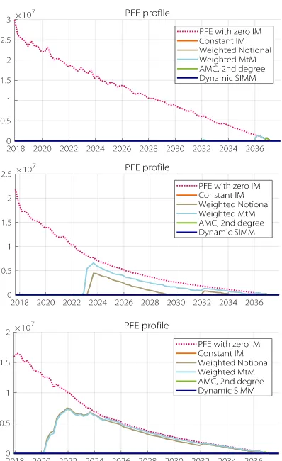
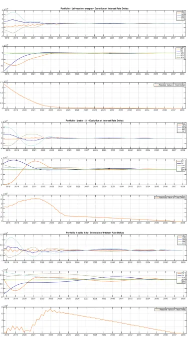
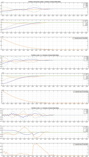
Our findings show that the accuracy of the three approximation methods is high when a bilateral netting set contains only interest rate receiver swaps or only interest rate payer swaps, no matter how large the bilateral netting set is or how long the residual maturity of the trades in the netting set is. The reason is that such netting sets have relatively simple dynamics (the future IM profile is mainly driven by the ageing of trades). As the Dynamic SIMM is generally seen to overcollateralize a bilateral netting set, we see that in such cases, residual exposure as measured by the Potential Future Exposure (PFE) measure is reduced to negligible levels under each IM approximation method. We see this from the top sub-figure in Figure 1-1.

As soon as the dynamics of the bilateral netting set become more complex (i.e., possibly offsetting sensitivities), the less the two weighted methods are able to track the benchmark, due to their incapability of capturing these dynamics well. Consequently, we see that the PFE profiles show increasingly residual exposure (the middle and bottom sub-figures in Figure 1-1). From a regulatory perspective, the Rabobank is more conservative when a non-zero residual exposure is assumed.

Under the more complex sensitivity dynamics conditions, the Weighted MtM method performs slightly better than the Weighted Notional method, due to the incorporation of the net-to-gross MtM ratio in the Weighted MtM method. This ratio has the capability to incorporate the netting set dynamics to some extent. However, for the effect of this ratio to become more profound and subsequently for the Weighted MtM method to track the Dynamic SIMM better, development of a multiplier on this net-to-gross MtM ratio should be considered. Also, some improvements on the used add-ons could be performed in order to improve performance of the Weighted MtM method. With these

improvement possibilities, the Weighted MtM method is recommended for implementation within Rabobank.

The AMC method on the other hand has potential to track the benchmark almost perfectly under more complex netting set dynamics as well. It must be noted, however, that the AMC method was scaled with a scaling function that improves the performance of the AMC significantly. However, due to the specific Brownian Bridge that the Rabobank has currently, there should be some adaptions in order to implement the AMC method. This puts a burden on the implementation procedure and therefore, the AMC method is less suited for the Rabobank with their current systems.

Page | 3

1

Introduction

The weaknesses of the global financial system were exposed during the financial crisis of 2007-2009. Especially the financial linkages and interdependence between large financial institutions were highlighted negatively. The underlying risk in these interconnections was mostly posed by the over-the-counter (OTC) derivatives market. The domino-effect that regulators feared, was almost realized after large counterparty exposures accumulated between market participants. Additionally, the risk stemming from such opaque and extremely complex financial interconnections was subject to risk management practices that were not mature enough to deal with this level of complexity. It went unnoticed that such constructs allowed for a build-up of extreme leverages. After September 2008, a different view towards counterparty credit risk and opaque multilateral constructs assisted by OTC-derivatives, was taken. The rest of this chapter explains briefly the regulatory reforms of the OTC derivatives market as a response to the financial crisis events and the outcomes of these reforms, which are shaped mainly into central counterparty clearing obligations and collateral margin regulatory frameworks.

1.1

Regulatory reforms

Some regulatory measures taken before the financial crisis prevented to a large extent that the feared domino-effect became reality. After the bankruptcy of Lehman Brothers, many of its counterparties were protected against the default due to collateral that Lehman Brothers posted under the regulatory requirements at that time. Additional collateral was posted by Lehman Brothers for the clearing of more than 60,000 OTC derivative contracts at LCH.Clearnet, thereby further dampening the financial default shock wave. After events like the Lehman bankruptcy, the attitude towards counterparty credit risk changed as the financial community realized the importance of this type of risk and the mitigation thereof.

The potential for systemic risk generated by the OTC derivatives market raised the interest of regulatory bodies and led to discussions at the G20 Summit in Pittsburgh on September 26th _{2009 and subsequently} to the development of regulation towards minimizing this type of risk. From the end of 2012 onwards, regulators required financial market participants to trade standardized OTC derivative contracts on exchanges or electronic trading platforms and that such transactions should be cleared through central counterparties. Additionally, OTC derivative contracts should be reported to trade repositories. Other derivative contracts, which are not centrally cleared became subject to higher capital requirements (European Union, 2012).

Page | 4

required to post initial and variation margins to each other in order to replicate the effect of CCPs' risk exposure management and the netting of exposures. This is termed bilateral margining, which is the focus of this thesis.

1.2

Problem setting

Within this new regulatory context, Rabobank is in need of modelling future initial margin (IM) for bilaterally collateralized OTC trade netting sets to be able to determine counterparty credit risk over the entire lifetime of a bilateral netting set. Because Rabobank assesses that ISDA’s upcoming Standard Initial Margin Model (SIMM, a sensitivity-based model) will become the market standard for calculating IM, the future IM forecast should be based on SIMM. Therefore, the main problem statement is:

How can the Rabobank forecast future IM based on SIMM in the most effective way?

This problem can be broken down into the following sub-questions:

 RQ1) What are the characteristics and regulatory requirements related to bilateral collateral exchange?

 RQ2) What are the challenges for Rabobank in implementing a SIMM forecasting methodology?

 RQ3) How is Potential Future Exposure defined?  RQ4) What are alternatives for modelling future SIMM?  RQ5) What is the most effective model?

1.3

Scope of research

Our research will focus on developing an effective method for forecasting future SIMM. The scope of research regarding this goal is to first develop a benchmarking model that will forecast SIMM based on future sensitivities (this future sensitivities model will not be implemented due to its computational infeasibility and serves merely as a benchmark, see discussions in the next chapters) and to subsequently develop approximation models for future SIMM from which the performance will be benchmarked against the benchmark model. From the approximation methods, the most effective method based on performance will be selected as a potential candidate for implementation at Rabobank. In determining the effectiveness of the forecasting methods, the impact of each method on the potential future exposure (PFE) will be used as graphical representation of the method performance. Rabobank uses the PFE for limit management purposes (i.e., to control counterparty future exposures).

OTC

Trade

Bilateral IM and VM Margining with CCP _{using CCP rules}

Standard Derivative Non-Standard Derivative

Page | 5

In order to be able to perform future SIMM simulations in an isolated environment (isolated from Rabobank’s daily production environment), the author created a Matlab experimental environment for this research that is capable of simulating netting set MtM valuations in the same way as Rabobank’s current Monte Carlo simulation engine. As the main product in Rabobank’s counterparty portfolios is the vanilla interest rate swap, the scope of our research will be experimental netting sets containing only this linear product. The Matlab experimental environment is therefore also confined to vanilla interest rate swaps (and also forward rate agreements1_{). Furthermore, the experimental bilateral netting sets will} be single-currency (EUR), for simplicity purposes facilitating analysis.

Finally, the thesis focuses mainly on the regulatory frameworks and regulations that apply to the EU (EMIR). As mentioned, the focus of this work are the requirements related to non-centrally cleared OTC derivative transactions. Transactions that clear through CCPs are out of scope.

1.4

Document Structure

The document structure is as follows. Chapter 2 discusses the characteristics of bilateral margining and some main regulatory points related to this type of margining, thereby answering RQ1. Chapter 3 treats the challenge related to forecasting future IM and focuses on answering RQ2. Chapter 4 discusses how exposure is modelled and how collateral plays a role in it. By defining PFE in this chapter, we are answering RQ3. Chapter 5 outlines the benchmark model and the three approximation models and the reasoning behind the models to answer RQ4. In Chapter 6, we provide the research setup and the experimental portfolios, which are employed in our Matlab environment to come up with the research results provided in Chapter 7. Ultimately, we answer research question RQ5 and our overall research problem in Chapters 8 (Discussion) and 9 (Conclusions) and we finalize the thesis with future research recommendations in Chapter 10.

1 _{Interest rate swaps can be seen as a cascade of multiple forward rate agreements. Therefore, being capable of simulate MtM}

Page | 6

2

Bilateral Margining and Regulations

The Working Group on Margin Requirements (WGMR) -a joint initiative of the Basel Committee on Banking Supervision (BCBS) and the International Organization of Securities Commission (IOSCO)- have put efforts into developing a framework that addresses the margin requirements related to non-centrally cleared OTC derivative contracts (ISDA, n.d.).This framework initiative is being translated into law by the individual regulatory authorities across jurisdictions. At this point, the US and EU authorities are implementing regulatory acts for these margins. In the US, such margin requirement regulations fall under the Dodd-Frank Act Title VII and are developed by the US Commodity Futures Trading Commission (CTFC) (Miller & Ruane, 2013). In the EU, these regulations are established by the European Market Infrastructure Regulation (EMIR) (O'Kane, 2016).

As mentioned above, many counterparties were protected to some extent from the Lehman Brothers' bankruptcy due to the fact that there were already some margin requirements present at that time. Requirements regarding the initial margin were existent as so-called independent amounts (IA) and fell under the Credit Support Annexes (CSAs), which were part of ISDA Master Agreements applicable to OTC derivative contracts. ISDA Master Agreements are the legal foundation of the OTC derivatives market and a CSA defines the overall amount of collateral that counterparties must deliver to each other, based on the specifics of the trade contract. The IAs were already part of these CSAs since the earliest days of the collateralized OTC derivative market, which dates back to the late 1980s (ISDA, 2010, p. 6). Although more formally applicable to exchange traded derivatives than OTC derivatives, requirements on the variation margin were always part of the Credit Support Balance in the CSAs. So, if the margin requirements already existed in some form, why was the bankruptcy of Lehman Brothers leading to financial distress at their counterparties and at the counterparties of their counterparties? The main issue at that time was that collateral received could be rehypothecated by the receiving party, as is the case with variation margin (discussed below). When that party defaults, counterparties who (over-) collateralized their exposure to the defaulting party will then see a recovery rate on their posted collateral of (significantly) less than 100%. This leaves the counterparties unsecured, potentially putting them at financial distress and triggering a domino-effect of defaults. Regulators now focus on redefining the variation margin collateral and on this rehypothecation issue and pose that next to a variation margin, an initial margin should be exchanged (bilaterally) for non-centrally cleared OTC derivative transactions and this collateral must be segregated at a third party account, thereby limiting rehypothecation to very specific conditions.

In the EU, shaping of the procedures for bilateral collateralizing of OTC trades comes from the BCBS and IOSCO initiative (Basel Committee on Banking Supervision, 2015) that led to the establishment of Article 11(15) of Regulation (EU) No. 648/2012 (EMIR)2 _{and the subsequent framework that} implements that Article (EIOPA, EBA & ESMA, 2016). As mentioned in the Introduction, the focus of our research is on the OTC market reforms’ collateral requirements. One of the key principles and requirements under the new regulations is that “all financial firms and systemically important non-financial entities (“covered entities”) that engage in non-centrally cleared derivatives must exchange initial and variation margin as appropriate to the counterparty risks posed by such transactions” (Basel

Committee on Banking Supervision, 2015, p. 5). The scope of the new margining requirements are financial counterparties and so-called NFC+ (non-financial counterparties with outstanding derivative transactions with a gross notional amount exceeding €1 billion for credit and equity derivatives or €3 billion for interest rate, FX, and commodity transactions). Under the new EMIR collateral requirements, the NFC+ counterparties have the same obligations as the financial counterparties. Below, the specifics of regulations for the two types of collateral will be discussed for the EU jurisdiction.

2 _{Regulation (EU) No. 648/2012 of the European Parliament and of the Council of 4 July 2012 on OTC derivatives, central}

Page | 7

2.1

Variation Margin

Under the new regulations the goal of VM is to provide the in-the-money party with sufficient collateral to cover the contract loss in case the out-the-money counterparty defaults, under the assumption that the defaulting counterparty provides a recovery rate of zero. VM is exchanged with a relatively high frequency (e.g., daily). First, netting is applied over all the contracts between the same two counterparties. Then, the netting value is determined based on market valuation. If this contract netting market value makes a counterparty in-the-money, then that party is protected. Thus, the VM must cover the maximum (end-of-day) loss that an in-the-money party can face due to the default of the counterparty. The mechanics related to VM are then such that the in-the-money counterparty is always holding the VM collateral and is allowed to rehypothecate this collateral. As soon as the market value of the contract shifts in favour of the other party (i.e., the in-the-money counterparty becomes out-the-money), then the VM collateral changes party.

The amount of VM collateral depends on factors such as the creditworthiness of parties (through Credit Valuation Adjustments (CVAs) on the mutual contract portfolios) and mutual contract portfolio discounting factors. Also, there may be subjectivity in determining the market value of some trades in the netting set, due to their character (like exotics or illiquid trades). This all may lead to a different valuation of the netting contracts by the two counterparties involved, thereby providing potential for disputes. For such dispute purposes, BCBS and IOSCO state that covered entities “should have rigorous and robust dispute resolution procedures in place with their counterparty before the onset of a transaction” (Basel Committee on Banking Supervision, 2015, p. 15).

Furthermore, a minimum transfer amount (MTA) can be agreed between counterparties. The regulators set the maximum MTA at €500,000 to enhance operational practicality. There is also a possibility for a threshold that allows for a maximum amount of VM uncollateralized exposure. This threshold can be agreed upon in the CSA between the counterparties. No VM has to be posted until the threshold amount is reached. When the exposure exceeds this threshold, the difference between the exposure and the threshold is posted to the in-the-money counterparty. However, upcoming regulations for VM require a zero threshold. Because of the one-way posting of VM, the overall market liquidity is not affected. The liquidity shifts from the posting counterparty to the receiving counterparty, creating a liquidity zero sum.

Page | 8 Table 2-1. The phasing of VM regulatory requirements.

Date of implementation VM specifics

1 September 2016

Every non-cleared OTC contract that is executed after 1 September 2016 between two covered entities, both with an average notional amount exceeding €3.0 trillion in non-centrally cleared transactions across March, April, and May 2016, is under VM margining requirements.

1 March 2017 From this date onwards, all covered entities are required to exchange VM.

2.2

Initial Margin

The IM collateral, on the other hand, is used to cover losses in the case the non-defaulting party faces a replacement cost of the joint contracts that is higher than the latest contract valuation (and thus exceeds received VM) that took place before the default of the counterparty. So, in the time between the latest valuation (and receipt of VM) and default of the counterparty, market movements may have increased exposure of the non-defaulting party and now this higher potential loss is uncovered by previously posted VM collateral. The time period between the last receipt of VM and the closing out of the bilateral netting set is called the Margin Period of Risk (MPOR). In contrast to VM, IM is posted two-way. Whether the non-defaulting party is in-the-money or out-the-money, it has received IM. When a counterparty defaults, it must return received IM to the non-defaulting party in full. This is possible, because IM is segregated. In case the loss occurs to the defaulting party, both counterparties receive back their IM collateral. The principle here is that the defaulting party pays the contract replacement costs (O'Kane, 2016).

IM collateral is posted by both counterparties to a third-party, custodian account so that IM is segregated and can only be rehypothecated under specific conditions. These conditions occur in the case when a corporate customer or non-financial company that post IM give permission to the IM receiving party that the collateral can be rehypothecated and only for hedging purposes of their joint netting set. In such cases, the receiving party with the rehypothecation permission, must inform their customer that the IM is rehypothecated and the amount that has been rehypothecated. Even when permission for rehypothecation is granted by the customer, the counterparty is responsible for protecting the rights of their customer.

Furthermore, there is a threshold for IM posting, set out by regulators. The maximum IM uncollateralized exposure that is allowed, is set at €50 million. When exposure builds up to this amount, no IM has to be posted. When the threshold is exceeded, the difference between the exposure and the threshold is posted as IM. Counterparties may agree a different threshold in the CSA, as long as it does not exceed €50 million. Next to the IM threshold, there is an IM minimum transfer amount. This amount is set at a maximum of €500,000. Again, the counterparties are able to agree on a different minimum transfer amount, as long as it does not exceed €500,000. To avoid the possibilities of counterparties creating new entities in order to use the thresholds multiple times and build excessive uncollateralized exposures, the regulators have set the thresholds to apply on a consolidated group basis.

Page | 9

decomposed into a physical FX transaction and a series of interest rate payments, the FX leg of the trade does not fall under the IM margining requirements.

As with the VM requirements, there are phase-in time periods for IM collateral requirements. The phase-in is related to the outstanding notional amount of non-centrally cleared transactions. The timeline for IM introduction is given in Table 2-2. It should be noted that the outstanding notional amounts of FX transactions, which are exempted from IM margining, are considered when determining the thresholds for phase-in of the IM requirements. Unlike with VM, there is no liquidity zero sum with IM posting. Exchange of IM collateral will have an impact on the overall liquidity of the financial markets.

Table 2-2. The phasing of IM regulatory requirements.

Date of implementation IM specifics

1 September 2016 – 31 August 2017 All covered entities with outstanding non-centrally cleared transactions with a monthly notional amount exceeding €3.0 trillion are required to exchange IM.

1 September 2017 – 31 August 2018 All covered entities with outstanding non-centrally cleared transactions with a monthly notional amount exceeding €2.25 trillion are required to exchange IM.

1 September 2018 – 31 August 2019 All covered entities with outstanding non-centrally cleared transactions with a monthly notional amount exceeding €1.5 trillion are required to exchange IM.

1 September 2019 – 31 August 2020 All covered entities with outstanding non-centrally cleared transactions with a monthly notional amount exceeding €0.75 trillion are required to exchange IM.

1 September 2020 – 31 August 2021 All covered entities with outstanding non-centrally cleared transactions with a monthly notional amount exceeding €8.0 billion are required to exchange IM.

2.2.1 Calculating Initial Margin at t0 (the regulatory IM)

Even though the focus of our research is on forecasting future IM collateral (based on SIMM), the first step is to determine IM at t0 (with which the forecasted IM at t0 should reconcile, more on this in subsequent chapters). For calculating this regulatory IM at t0, regulations (EIOPA, EBA & ESMA, 2016) allow three approaches:

 The Standardized Approach (SA), which is based on add-ons.

 Own developed initial margin model (based on Internal Model Method) which is developed by one or both counterparties, or by a third party. This model shall be based on a one-tailed 99 percent confidence interval over an MPOR of at least 10 business days. Furthermore, the calibration of the model should use at least three years of data and not exceed five years of data, from which at least 25% should be stressed data.

Page | 10

As mentioned, Rabobank’s preferred choice of the three models for calculating IM at t0 is SIMM3_{. At} this point, the SIMM as a method for calculating IM is still under review in Europe. In the US and Japan, the method went live. Because of these two globally large financial powers and global trading, it will be a matter of time before the SIMM becomes a global standard for initial margin calculation. Being at the forefront and getting the SIMM implementation right can be a major business opportunity for financial institutions.

2.2.2 Allowed collateral types

For VM and IM collateral to reduce counterparty credit risk during adverse times, it is necessary for the collateral to be stable in value even during times of financial stress. Regulators want to avoid that the collateral used is correlated to the default of a counterparty. To reduce such correlation risk, the collateral should be the most highly liquid assets. However, there is a trade-off between the liquidity of collateral and the overall market liquidity. Due to the fact that IM is segregated after posting, the overall liquidity of the financial markets is reduced because large numbers of highly liquid assets are taken out of circulation. To reduce such a strain in liquidity, regulators have determined a variety of eligible collateral. Compensating for liquidity of the eligible collateral, so-called collateral haircuts to the asset’s value are introduced for each type of collateral. The haircuts are presented in Table 2-3 (Basel Committee on Banking Supervision, 2015). The table shows that it is possible to hold assets as collateral with a different underlying currency than the one of the trades in the netting set. In such cases, the haircut is increased with 8% of the asset’s market value (last row in Table 2-3).

Table 2-3. Standardized haircut schedule.

Asset Class Haircut (% of market value)

Cash in same currency 0

High-quality government and central bank securities: residual maturity less than one year

0.5 High-quality government and central bank securities: residual maturity between one and five years

2

High-quality government and central bank securities: residual maturity greater than five years

4

High-quality corporate\covered bonds: residual maturity less than one year

1 High-quality corporate\covered bonds: residual maturity greater than one year and less than five years

4

High-quality corporate\covered bonds: residual maturity greater than five years

8 Equities included in major stock indices 15

Gold 15

Additional (additive) haircut on asset in which the currency of the derivatives obligation differs from that of the collateral asset

8

3 _{A comparison between calculations for IM at t}

0 under SIMM and Standardized Approach is presented in Appendix A for an

Page | 11

3

Challenges for Rabobank

Rabobank has a comprehensive risk management philosophy that has led to an integrated market and counterparty credit risk policy, control and reporting framework. Within that integrated framework, Rabobank has a Counterparty Credit Risk (CCR) sub-framework that is geared towards the analysis and quantification of counterparty credit risk. Within CCR, Monte Carlo analysis is the essential technique to analyse and quantify market (risk) factor movements dynamically and their impact on the financial derivatives portfolio that the bank holds. Based on these movements, Rabobank is able to compute:

1. The Potential Future Exposure (PFE), which is a 97.5 percentile of the distribution of exposures4 _{at a given time point. This risk measure is used to check whether a trade with a} counterparty can be executed within set limits (i.e., limit management).

2. Exposure at Default (EaD), which is a risk measure used for regulatory (RC) and economic capital (EC) calculations.

As mentioned in the first chapter, a graphical representation of performance of the SIMM forecasting methods will be provided by showing the impact of the methods on the PFE profile. At this point, the Rabobank's CCR framework includes a precursor of IM (Independent Amount), which is modelled as a linear balance throughout the lifetime of a bilateral netting set. In order to see the impact of new IM regulations on exposure profiles, more accurate modelling is needed than a linear model.

3.1

Forecasting future IM

Figure 3-1 shows the difference between IM at t0 (the new regulatory requirement) in subfigure A, and the future IM in subfigure B if we were to use the IMM to model future initial margin (as mentioned previously, we not use IMM, but we extend SIMM. The reason for showing the figure is merely to illustrate the complexity when IMM would have been used).

In Figure 3-1A, we see a portfolio value movement over the MPOR period depicted as scenarios and starting at t0. The 99th percentile Value-at-Risk (VaR) of the portfolio value movement over the 10

business day MPOR period, based on these value movement scenarios, represents the regulatory IM (i.e., the IM that our counterparties should post to us in order to cover our 99th _{percentile value change} of the portfolio at t0). In Figure 3-1B, we see that the MPOR period does not start at t0, but at a future

time point t. This means that we are forecasting IM in the case the counterparty defaults at time point t. With this approach a situation would be introduced where nested scenarios arise.

Simulating thousands of value movement scenarios for large and complex portfolios burdens computational resources, let alone simulating nested scenarios for such cases. Simulating future SIMM accurately would require simulation of future sensitivities within the mentioned nested model. Due to the complexity and computational infeasibility, Rabobank has decided not to base their SIMM forecasting on IMM, but rather to use an approximation method. The challenge lies in developing an approximation method that is performing well in terms of precision of the future SIMM forecast, while at the same time being an easy to implement method. The challenge can be summarized as an accuracy versus complexity trade-off.

4 _{Exposure is defined as:}

Page | 12

Netting set value t0

MPOR

(10 business days)

t₀ Netting

set value

t

MPOR

(10 business days)

t₀- IM Future IM at time point

t

99% VaR

99%

VaR

99% VaR

99% VaR 99%

VaR

A

B

Figure 3-1. A. Netting set market value movement over the MPOR period when MPOR starts at t0 (i.e., when the

counterparty defaults at t0. This is the regulatory IM).

B. Netting set market value movement between t0 and t and the subsequent market value movement during the

Page | 13

4

Modelling Exposure

In this chapter, the process of modelling counterparty exposure through time will be outlined. Before we proceed to the modelling process, the exposure and how it is defined will be explained first.

4.1

Potential Future Exposure (PFE)

Generally, exposure can be defined as:

𝐸𝑥𝑝𝑜𝑠𝑢𝑟𝑒 = max (𝑀𝑡𝑀, 0)

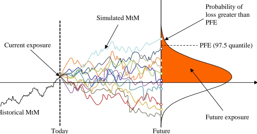
It is the positive value of the netted trade values in the counterparty portfolio or the so-called netting set. So, to be able to quantify exposure, the MtM of each individual trade in the portfolio throughout time has to be simulated first and then netted. The positive part of the resulting distribution of netted MtM represents the exposure. Figure 4-1 shows the future exposure based on simulated evolutions (scenarios) of a netting set. For our research, the exposure will be quantified by a 97.5% Potential Future Exposure (PFE). The 97.5% PFE level is also shown in Figure 4-1. The formal definition of the uncollateralized PFE is:

𝑃𝐹𝐸_𝑡,𝑥%= (max(𝑀𝑡𝑀_𝑡, 0))_𝑥%

where MtMt is the fair value of the netting set and x represents the quantile level (in this case 97.5%).

With this level (quantile) of the PFE, it means that the PFE will be exceeded in 2.5% of the scenarios at each time point that the distribution is considered. However, the size of the loss within that 2.5% can be infinite.

Received collateral (like VM) is used to reduce the exposure. The collateralized PFE is expressed as:

𝑃𝐹𝐸𝑡,𝑥%= (max(𝑀𝑡𝑀𝑡− 𝐶, 0))𝑥%

Figure 4-1. Showing a graphical representation of the simulated MtM future evolutions (scenarios) of a netting set and the resulting future exposure (shaded area on the distribution graph. Also, the 97.5 quantile PFE is shown.

Future exposure PFE (97.5 quantile)

Future Today

Current exposure

Historical MtM

Probability of loss greater than PFE

Page | 14

where C represents the collateral balance, existing of VM and IM. To be able to measure future exposure, it is necessary to model future collateral. An important aspect in modelling collateral is the Margin Period Of Risk (MPOR).

4.2

Margin Period Of Risk (MPOR)

Between a margin call (a call to the counterparty for posting collateral) and the actual receiving of the collateral, some time may pass due to a dispute for example. Disputes related to collateral posting may arise, because it is very likely that both parties have different methods of calculating the collateral, thereby increasing the probability for a mismatch between the margin call and the amount of collateral the called-upon party believes it should post. During this time between the last posting of collateral and the dispute settlement, the party that is entitled to collateral may see a rise of the portfolio value at their side and thereby face an increased exposure. This settlement time period is also termed MPOR. Another example that may invoke an MPOR is a default of the counterparty. When the counterparty goes into default there will be an MPOR between their last collateral posting and the re-hedging of the portfolio by the non-defaulting counterparty. The MPOR can be depicted graphically as is done in Figure 4-2. In line with the Rabobank’s Counterparty Credit Risk (CCR) framework, the length of the MPOR is defined to be 14 calendar days (or 10 business days). For the remainder of this thesis the 14-day MPOR will be used.

4.3

Collateral Modelling

Generally, the collateral balance at time t is a function of MtM at time t-MPOR. Furthermore, to increase operational convenience there are two types of thresholds related to collateral posting, which are taken up in the CSAs between counterparties.

4.3.1 Exposure threshold

The first type of threshold is a limit on how much unsecured counterparty exposure can be built up before collateral posting is required. For example, if the threshold is set at 5 million by a counterparty, the exposure of 4 million at that party will not lead to a margin call from that party to its counterparty. Only when the exposure has accumulated to a value equal to or larger than 5 million, collateral calls will be made. In practice, it is very likely that two counterparties have different thresholds.

4.3.2 Minimum Transfer Amount (MTA)

The second type of threshold is a minimum limit on the amount of collateral to be posted when the exposure threshold has been reached. This threshold is called the Minimum Transfer Amount (MTA). There are some rounding rules applicable to the MTA, which are specified in CSAs. Like the exposure threshold discussed above, the MTA can be different for both counterparties.

Last collateral posting

Default of counterparty

Closing out netting set

Page | 15 4.3.3 Collateral balance

The collateralized counterparty exposure can generally be denoted as:

𝐸𝑥𝑝𝑜𝑠𝑢𝑟𝑒 = max (𝑀𝑡𝑀 − 𝑉𝑀 − 𝐼𝑀, 0)

where IM represents the received IM. From this the 97.5% PFE at each time point t follows:

𝑃𝐹𝐸_𝑡,97.5%= (max(𝑀𝑡𝑀_𝑡− 𝑉𝑀_𝑡− 𝐼𝑀_𝑡, 0))_97.5%

So, to find the exposure we need to find the evolution of the collateral balance VMt+ IMtthroughout

time. This expression makes again clear the purpose of modelling future IM; otherwise it is not possible to obtain the PFE. At this point, Rabobank does not have a model to be able to model IM throughout time (future IM). As part of our research, specific alternatives are presented in Chapter 5.

4.3.4 Obtaining the MtM at non-simulation dates

Next to the IMt-term, the MtMt-MPOR-term in Equation Error! Reference source not found. is not

directly available by sampling the MtMs at the simulation grid dates. In other words, the MtMt-MPOR

-term is not a simulated point, unless the simulation grid is extremely granular. This is not possible due to computational restraints. With a coarsely grained simulation grid, the MtMt-MPOR-term has to be

interpolated between the simulated points in some way. The interpolation technique used is the Brownian Bridge. The Brownian Bridge gives a conditional probability distribution of a Wiener process

Page | 16

5

Future SIMM forecasting model alternatives

This chapter will discuss considered alternative models for forecasting future SIMM. Generally, a distinction can be made between three types of models that have potential to this end (Gregory, 2015) mentions these types for quantification of credit risk exposure, so they are equally well applicable to forecasting future SIMM):

 Parametric approaches (for example, add-on based approximations).

 Semi-analytical methods (approximating distributions based on some conditions, like the values of MtM at specific points or the values of risk drivers at specific points).

 Monte Carlo simulation of future SIMM (the most complex and computationally heavy methods, but highly accurate).

It is clear from the three model categories that there is a trade-off between high computation and time consumption, and lower accuracy in forecasting. To be able to evaluate the performance of the developed alternatives for forecasting future SIMM, it is necessary to first develop a benchmark to which the performance of the approximation models can be compared. To obtain the best possible accuracy, the benchmark model will be one of the Monte Carlo simulation category. The benchmark model is not considered for implementation at the Rabobank. It is merely used for development and evaluation of the approximation models. Next to the benchmark model, we develop two models that use a parametric approach to forecast future SIMM, and one model that fits the semi-analytical methods category.

Additionally, there are some requirements for the alternative IM forecasting models (Anfuso. et al., 2017):

Req1.The IM at t0 should reconcile with the regulatory required IM at t0 as obtained by the SIMM

method (i.e., IM(paths, t0) = SIMM(t0) ∀𝑠, see Chapter A for the t0-IM calculation).

Req2.The calculated IM should segregate trades from different asset classes, so there should be no netting benefit across asset classes (i.e., 𝐼𝑀(𝑝𝑎𝑡ℎ𝑠, 𝑡) = ∑𝐾𝑘=1𝐼𝑀𝑘(𝑝𝑎𝑡ℎ𝑠, 𝑡) ∀𝑘 𝑎𝑛𝑑 𝑠, where k

represents the asset class) (Basel Committee on Banking Supervision, 2015).

Req3.To minimize computational burden, the future SIMM forecasting model should use as inputs the simulation outcomes from currently available systems.

5.1

Dynamic SIMM – the benchmark model

The first model to be treated is the model that will be used as the benchmark for the approximations. This model is based on SIMM. The difference between the t0-value obtained from SIMM and the

future-t SIMM-values lies in the use of dynamic sensitivities. So, where the t0 SIMM-value is obtained by

using today’s sensitivities, we plug in simulated sensitivities at future time points into SIMM to obtain the future SIMM forecast. This model will be called the Dynamic SIMM throughout the rest of this thesis.

Page | 17

The sensitivities that SIMM uses as input for interest rate products are partial durations for the following tenor points (ISDA, 2017): 2W, 1M, 3M, 6M, 1Y, 2Y, 3Y, 5Y, 10Y, 15Y, 20Y, and 30Y. As seen in Figure 5-1, the simulated tenor points differ from SIMM’s requested input tenor points. To transform our tenor grid to that for SIMM, linear interpolation will be used on our partial durations (obtained from simulation). This interpolation procedure is in line with the ISDA’s Risk Data Standards for SIMM (ISDA, 2017).

5.2

Weighted Notional Model

In order to establish practical approximations, models based on simulation of future SIMM from dynamic deltas cannot be considered, as these are impractical due to the computational burden. We need to come up with alternative models that have the potential to approximate the Dynamic SIMM, while not using simulated deltas and at the same time satisfy requirements Req1-Req3. In order to satisfy requirement Req1, we use the t0-IM value as obtained by SIMM, rather than SA. Because we

use Dynamic SIMM as the benchmark model, it is natural to use t0 IM values as obtained by the t0

SIMM. Henceforth, all the t0 IM values will be obtained by the t0 SIMM (i.e., by plugging in t0

sensitivities into SIMM).

After obtaining the t0 IM value, the next step is to determine how this value is to be amortized over the

lifetime of a counterparty portfolio. For this, we consider the ageing of the trades within the portfolio. Correspondingly, we need to determine some sort of value associated with the still alive trades in the portfolio at each future time point, while at the same time not creating any computational burden and using the outputs from the currently available systems (requirement Req3). The simplest values we can come up with are the notional amounts of the trades. These are available in the current system. To capture the ageing of trades we can simply use (regulatory) add-ons. With the proposed elements, we propose the following simple IM amortization scheme, based on weighting the notional with add-ons:

𝐼𝑀_𝑊𝑁(𝑡) = ∑ 𝐼𝑀_𝑘(𝑡₀)

𝑘

[ ∑ |𝑁𝑜𝑡𝑖𝑜𝑛𝑎𝑙𝑖𝜖𝑘 𝑖(𝑡)| ⋅ 𝐴𝑑𝑑𝑂𝑛𝑖(𝑡)

Page | 18

where WN indicates the amortization method (Weighted Notional), t indicates time, k indicates the asset class, and i indicates the trades within a single asset class, subject to IM requirements. By separating the trades and t0-IM per asset class, we satisfy requirement Req3.

5.3

Weighted MtM Model

With the next model, we aim to capture portfolio dynamics better than is possible with Equation 5-1. The simplest dynamic that we can capture additionally is the netting benefit of trades within a portfolio. Therefore, we extend the Weighted Notional Method by introducing MtM into Equation 5-1. Future MtM simulations of trades are also available from the currently used system at Rabobank, so we are still satisfying requirement Req3. To include the effect of the netting benefit by means of MtM, we mimic the Standardized Approach, as described in Chapter A. This means that the netting benefit can be up to 60%. With the discussed addition, we propose the following amortization method:

𝐼𝑀_𝑊𝑀(𝑡, 𝑠) = ∑ 𝐼𝑀_𝑘(𝑡₀)

𝑘

[

∑ |𝑁𝑜𝑡𝑖𝑜𝑛𝑎𝑙_𝑖(𝑡, 𝑠)| ⋅ 𝐴𝑑𝑑𝑂𝑛_𝑖(𝑡) ⋅ (0.4 + 0.6 ∙ [∑ 𝑀𝑡𝑀𝑖 𝑖(𝑡, 𝑠)]+

∑ [𝑀𝑡𝑀𝑖 𝑖(𝑡, 𝑠)]+) 𝑖∈𝑘

∑𝑖∈𝑘|𝑁𝑜𝑡𝑖𝑜𝑛𝑎𝑙𝑖(𝑡0)| ⋅ 𝐴𝑑𝑑𝑂𝑛𝑖(𝑡0)⋅ (0.4 + 0.6 ⋅[∑ 𝑀𝑡𝑀𝑖 𝑖(𝑡0)] +

∑ [𝑀𝑡𝑀_𝑖(𝑡₀)]+

𝑖 )

] 5-2

where WM indicates the amortization method (Weighted MtM), t indicates time, s indicates senarios, k

indicates the asset class, and i indicates the trades within a single asset class, subject to IM requirements. Comparing Equation 5-2 to Equation 5-1, we see that the Weighted MtM method is scenario-dependent, whereas the Weighted Notional method is not. The reason is that Rabobank’s system simulates MtM at different time points as well as for different scenarios. Just like the Weighted Notional method, the Weighted MtM method satisfies requirement Req2.

5.4

American Monte Carlo

Here, we propose a model that is of the semi-analytical type, which is based on the seminal publication from Longstaff & Schwartz (2001). The method has been known as American Monte Carlo and it is based on least-squares regression. This method is proposed by Anfuso et al. (2017) to forecast future SIMM.

The American Monte Carlo (AMC) method for forecasting future SIMM is based on determining the local volatilities via least-squares regression with a polynomial basis. Generally, the AMC methodology reuses the MtM simulation paths at each time point t to determine the local distribution of ΔMtM(t, t+MPOR, paths). The IM can then be expressed as:

Page | 19

Longstaff-Schwartz argumentation working towards the situation in Equation 5-3, we can express the second moment of the nested distributions as (only if μ=0):

𝜎2_{(𝑡, 𝑠) = 〈(∆𝑀𝑡𝑀(𝑡, 𝑠))}2_{|𝑀𝑡𝑀(𝑡, 𝑠)〉 = ∑ 𝑎}

𝜎,𝑛𝑀𝑡𝑀(𝑡, 𝑠)𝑛 𝑛

0

5-4 where ΔMtM(t,s) is short for ΔMtM(t, t+MPOR, paths). The right hand side of the Equation can be

obtained by least-squares regression with a polynomial basis as shown by Longstaff and Schwartz (2001) and n represents the polynomial degree. It has been established that a second-degree polynomial gives the best results for determining the local variances (Caspers et al., 2017), so n=2 in our case. Here, we have chosen our filtration 𝓕t to consist of conditional value in terms of MtMs, but we can also adapt the risk drivers to the filtration. Anfuso et al. (2017) and Caspers et al. (2017) argue that this is a more precise approach. However, for simplicity we use conditioning on MtM. Now, we can forecast future IM by:

𝐼𝑀_𝑅,𝑘𝑈 _{(𝑡, 𝑠) = 𝛷}−1_{(0.99, 𝜇 = 0, 𝜎 = 𝜎(𝑡, 𝑠)) 5-5}

Where Φ-1(x,μ,σ) represents an inverse cumulative normal distribution, evaluated at confidence level x, and R indicates received IM (on purpose we make a distinction between received IM and posted IM, because of asymmetry of the distribution). We are only interested in the received IM in the rest of this thesis, so we disregard the posted IM and refer to the received IM when mentioning IM. In Equation 5-5, The U in the subscript indicates that the future IM profile is unnormalized. In order to satisfy requirement R1, we need to normalize the function in Equation 5-5 with the following normalization function:

𝛼0= √

𝑀𝑃𝑂𝑅 10𝑑 ⋅

𝐼𝑀_𝑡=0

∑𝐾𝑘=1𝑄_0.99(∆𝑀𝑡𝑀𝑘(0, 𝑀𝑃𝑂𝑅))

=∑ 𝑆𝐼𝑀𝑀𝑡=0,𝑘

𝐾 𝑘=1

∑𝐾 𝐼𝑀_𝑡=0,𝑘𝑈 𝑘=1

5-6

With Equation 5-6, we are able to reconcile our unnormalized model from Equation 5-5 with the SIMM-value that we obtain for t=0, in the following way:

𝑆𝐼𝑀𝑀(𝑡, 𝑠) = 𝛼0∑ 𝐼𝑀𝑘𝑈 𝐾

𝑘=1

5-7

Anfuso et al. (2017) further propose in their publication that we use the following function to normalize Equation 5-5:

𝛼(𝑡) = (1 − ℎ(𝑡)) ⋅ √_{𝑀𝑃𝑂𝑅}10𝑑 ⋅ [𝛼_∞+ (𝛼₀− 𝛼_∞) exp −𝛽(𝑡) ⋅ 𝑡] 5-8

where β(t)>0 and h(t)<1, with h(t=0)=0 are functions to be calibrated (in our case two functions, but usually these represent four functions: each function is calibrated for receiving IM as well as posting IM). The 𝛼∞parameter is a constant and 𝛼0 is also a constant as defined in Equation 5-6. The

𝛼_∞parameter accounts for the long-term scaling level as t→∞. β(t) is a mean-reversion speed function that determines the transition from α(t=0) to 𝛼∞. The h(t) function can be used to reduce back-testing

exceptions (Anfuso et al., 2017) and make to IM forecasting model more conservative. Including the

α(t) function, this gives us the final SIMM forecast from the AMC method as:

𝑆𝐼𝑀𝑀_𝐴𝑀𝐶(𝑡, 𝑠) = 𝛼(𝑡) ∑ 𝐼𝑀𝑘𝑈 𝐾

𝑘=1

Page | 20

Calibration methods for the elements of the function in Equation 5-8 are discussed by Anfuso F. et al.

Page | 21

6

Research Setup

We select three representative bilateral netting sets as a starting point to obtain our results and perform the analysis. Representative means in this case that the three netting sets cover the characteristics seen in counterparty portfolios consisting of IRS trades only and have EUR as the only underlying currency, together with the characteristic that all the trades in the EUR bucket are exposed to the same yield curve (i.e., EUR 3M LIBOR).

The selection consists of two large netting sets (>250 trades), but with different compositions of receiver and payer IRSs and difference in the time to maturity, and a smaller netting set (<100 trades). Below, these three netting sets will be discussed in more detail. Also, we alter the ratios of payer to receiver swap within these netting sets later in this section to obtain a higher, more representative diversity of netting sets.

We have selected these three netting sets as a starting point for our analysis, because they have similar characteristics to most of Rabobank’s bilateral netting sets: single-currency, single underlying yield curve, and in which 80%-100% of the trades are IRSs. By choosing these sets and altering the payer to receiver swap ratios in an experimental setting, we are able to generalize the outcomes of our analysis over all such Rabobank bilateral netting sets.

6.1

Portfolio 1

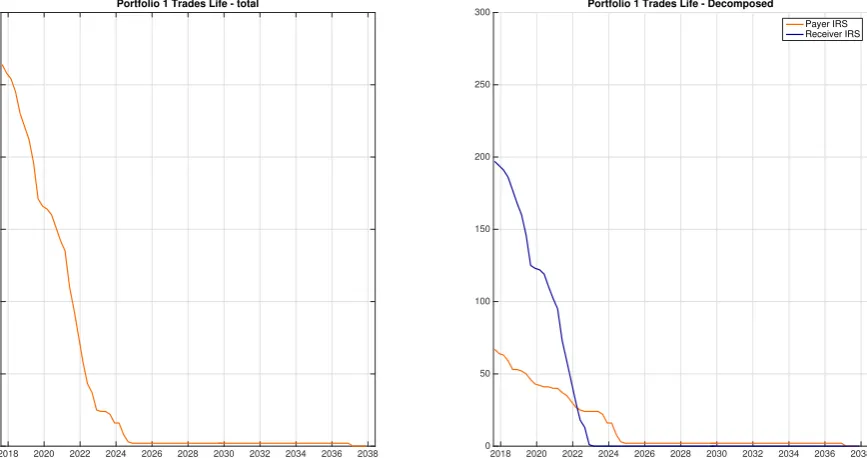
The first netting set (to be called Portfolio 1 throughout the remainder of this thesis) is a portfolio which contains 264 IRS trades. The ageing of trades and the composition of payer and receiver swaps within this portfolio is shown in Figure 6-1. From the right-hand graph in the figure, it can be seen that the t0 composition of this counterparty portfolio contains 197 receiver swaps and 67 payer swaps.

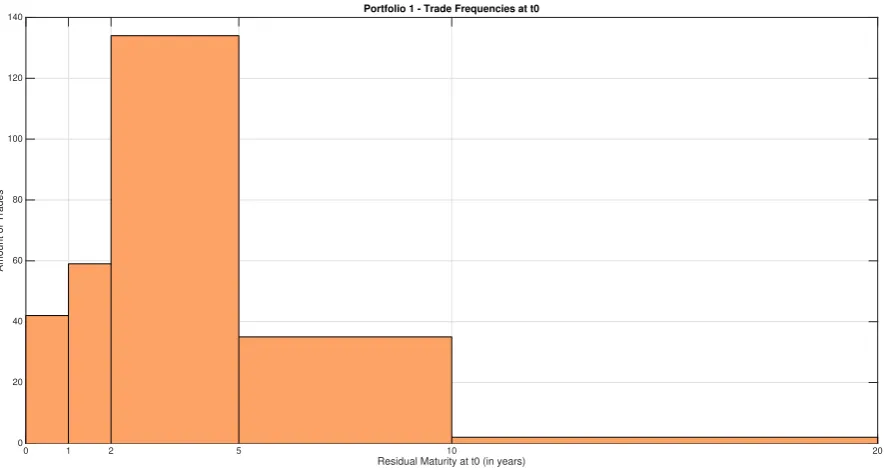
Figure 6-2 shows the composition of Portfolio 1 in terms of time-to-maturity at t0 (residual maturity at t0). We can see from the figure that most of the trades have a relatively short residual maturity (0-5 years). The portfolio has a low number of trades with a longer residual maturity as well (5-10 years) and even a few long residual maturity trades (10-20 years), but its number is negligable.

Page | 22 Figure 6-2. The number of trades in Portfolio 1 per residual maturity (at t0) category. The largest portion of the trades in the

counterparty portfolio have a residual maturity at t0 between 0 and 5 years.

6.2

Portfolio 2

The second counterparty portfolio (to be called Portfolio 2 throughout the remainder of this thesis) is a Portfolio with 275 IRS trades. Figure 6-3 shows the ageing of the trades and the composition of the portfolio in terms of receiver and payer swaps. We can see that this counterparty portfolio is an all-receiver swap portfolio.

Page | 23

Figure 6-4 shows the composition of the portfolio in terms of residual maturity at t0. Compared to Figure 6-2, Portfolio 2 has more trades in the mid- to long residual maturity region.

6.3

Portfolio 3

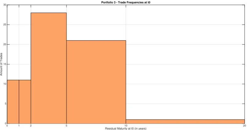
Portfolio 3 is the smallest counterparty portfolio of the three selected portfolios and contains 72 IRS trades, from which all are receiver swaps (Figure 6-5) and the largest portion of the trades has a residual maturity at t0 in the mid-region (2-10 years)(Figure 6-6).

Figure 6-5. Portfolio 3 evolution of trades through time. There is a total of 72 trades in the Portfolio at t0.

Figure 6-4. The number of trades in Portfolio 2 per residual maturity (at t0) category. The largest portion of the trades in the

Page | 24

6.4

Changing the payer-to-receiver swap ratio

The above-mentioned three counterparty portfolios have a limited range of payer-to-receiver swap ratios (i.e., Portfolios 2 and 3 are all-receiver swap portfolios and only Portfolio 1 has a non-zero amount of payer swaps). Changing the ratio allows for variation in delta profiles through time, as a higher payer-to-receiver swap ratio may create a more delta-offsetting position within a single portfolio. Therefore, we introduce in a systematic way some more portfolios to be able to capture the effects of delta exposure on the alternative future SIMM models.

The approach to expand the experimental portfolios systematically is to create new portfolios from the three portfolios in the way as described in the table below. All portfolio names for further reference are stated in each cell between parentheses.

Table 6-1. Experimental portfolio setup

All-receiver swap 25% payer swaps 50% payer swaps Large

portfolio, short-mid residual maturity

Portfolio 1 where all the payer swaps are

converted into receiver swaps

(Portfolio 1A)

Unaltered Portfolio 1

(Portfolio 1B)

Portfolio 1 where 65 of the 197 receiver swaps are converted into

payer swaps (Portfolio 1C) Large portfolio, mid-long residual maturity

Unaltered Portfolio 2

(Portfolio 2A)

Portfolio 2 where 69 of the 275 receiver swaps are converted into

payer swaps

(Portfolio 2B)

Portfolio 2 where 138 of the 275 receiver swaps are converted into

payer swaps (Portfolio 2C) Small portfolio, mid res. maturity

Unaltered Portfolio 3

(Portfolio 3A)

Portfolio 3 where 18 of the 72 receiver swaps are converted into

payer swaps

(Portfolio 3B)

Portfolio 2 where 36 of the 72 receiver swaps are converted into

payer swaps

(Portfolio 3C) Figure 6-6. The number of trades in Portfolio 3 per residual maturity (at t0) category. Most of the trades in the