University of Warwick institutional repository: http://go.warwick.ac.uk/wrap
This paper is made available online in accordance with publisher policies. Please scroll down to view the document itself. Please refer to the repository record for this item and our policy information available from the repository home page for further information.
To see the final version of this paper please visit the publisher’s website. Access to the published version may require a subscription.
Author(s): W. J. Lewis
Article Title: Computational form-finding methods for fabric structures Year of publication: 2012
Link to published article:
Computational form-finding methods for fabric structures by
Prof. W.J. Lewis Dip., Inz., MSc., PhD., CEng., MIStructE., FICE School of Engineering, University of Warwick, Coventry CV4 7AL
Tel: 024 76 523 138; Fax: 024 76 418 922
Email:
Date: 21st June 2008 Word count: 6111
No. of Figures: 7 No. of tables: 1
A review of computational form-finding methods for fabric structures Abstract
Form-finding is a process that determines the surface configuration of a fabric
structure under pre-stress. This process can be carried out using a variety of
numerical methods, of which the most common are: (i) transient stiffness, (ii) force
density, and (iii) dynamic relaxation. This paper describes the three methods,
discusses their advantages and limitations, and provides insights into their
applicability as numerical tools for the design of fabric structures. Further, it
describes various approaches to surface discretisation, and discusses consequences of
using ‘mesh control’ and elastic effects in the design of form-found surfaces. A brief
discussion of the general recommendations given in the European Design Guide for
1. Introduction
The design of a fabric structure differs from that used in conventional structural
design in that it has to determine the shape of the canopy under prestress. The
resulting surface geometry must satisfy the condition of static equilibrium and have as
uniform stress distribution as possible. For these highly flexible structures, the
process required to define their initial surface geometry is known as form-finding. As
a concept, form-finding is not generally understood, except by specialists working in
the area. Even then, the conviction that “I can build whatever shape I like” does arise
occasionally. This problem stems from the fact that architects and engineers are used
to dealing with structures of ‘known’ shape, i.e., rigid-type forms shaped at the outset
by aesthetic and functional considerations. It is, therefore, difficult to come to terms
with the fact that fabric structures are different; they adopt unique configurations
under loading; configurations that, quite literally, have to be found.
Prior to 1970, form-finding of tension membrane structures was carried out using
small-scale, physical models made of fabric or soap-film1. It was the design of the
Munich Olympic complex in 1972 that marked the departure from the exclusive use
of physical models in favour of computational form-finding and load analysis.
Currently, the three most commonly used computational form-finding methods, which
have been implemented in commercial software, are known as:
(i) transient stiffness
(ii) force density
(iii) dynamic relaxation.
In all cases, regardless of the approach/method used, the process involves iterative
Before discussing each of the methods in turn, it is worth noting that surface
discretisation, i.e., the representation of the continuum by a system of inter-connected
elements, is an important underlying factor influencing theoretical formulations and
implementations of form-finding methods, as well as the accuracy of the solution.
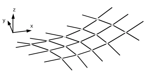
The simplest surface discretisation is achieved using a mesh of line, or cable elements
as shown in Fig. 1. In this case, the methodology adopted does not differ from that of
the analysis of a tensioned cable net. This type of surface discretisation is used in
each of the methods listed above, in order to explain their distinguishing features in a
consistent and clear manner.
2. Transient stiffness method
The transient stiffness method2,3 is based on small displacement theory that assumes
linear dependence of deflections upon forces applied to the structure. The surface,
discretised using line elements, forms a two-way system of cables intersecting at the
nodes (Fig. 1).
x y
[image:5.595.184.429.504.626.2]z
Fig. 1. Surface discretisation by line, or cable elements
The form-finding process starts with an assumed (guessed) surface configuration,
and summing up the contribution from each member sharing the same node, gives the
resultant internal force vector,
{ }
P~ .As the system is unlikely to be in equilibrium, the resultant internal force
{ }
P~ ≠{ }
0 ; itrepresents an out-of-balance, or residual force vector,
{ }
R ={ }
P~ . Therefore, if {δ} is the vector of nodal displacements corresponding to the residual force vector,{R}, and[K} is the global stiffness matrix, then it is possible to write:
[ ]
K{ } { }
δ = R (1)and determine the required displacements as:
{ }
δ =[ ]
K −1{ }
R (2)However, there is a problem with the direct use of the above equation. Unless the
initially guessed surface configuration is very close to the equilibrated, form-found
surface, the residual force vector {R} is likely to be large, and, therefore, the
calculated vector of nodal displacements {δ} is also large. This invalidates the
assumption of small displacements used in formulating [K]. Consequently, eqn.(2)
can only be satisfied through an iterative process of calculating incremental residual
forces and displacements, as explained below.
With k denoting the kth iterative step, the current geometry of the structure is denoted
by {X}k, and the stiffness matrix calculated on the basis of this geometry is [K]k. At
k=0, the residual force vector
{ }
R k can be calculated by resolving the internal forces at the nodes. In order to preserve the assumption of linear behaviour, a small proportionof this residual force vector, denoted as
{ }
∆
R k needs to be applied to find anincrement in nodal displacement vector,
{ }
∆δ . Thus, at the next iterative step:{ }
∆δ k =[ ]
K k{ }
∆R k−
+1 1 (3)
{ }
X k+1={ } { }
X k + ∆δ k+1 (4)The new geometry is used to calculate a new (updated) stiffness matrix,
[ ]
K k+1. Atthis point, a new residual force vector,
{ }
Rk+1 is found by resolving the forces again and a small proportion of it,{ }
∆R k+1 is applied to find the next increment in thedisplacement vector,
{ }
∆δ k+2 and the new (updated) geometry{ }
X k+2.The resulting iterative process of calculations continues until the residuals are reduced
to (almost) zero, i.e. until the static equilibrium is reached. Experience is needed in
selecting an appropriate value of
{ }
∆Rk. Its magnitude should be small enough toensure that the assumption of small displacements holds, and, at the same time, large
enough the give a reasonable rate of convergence.
The numerical procedure presented above is known as the 'transient stiffness method.’
Accordingly, the stiffness matrix
[ ]
K k is referred to as a transient stiffness matrix, or instantaneous stiffness matrix. Although the numerical procedure is formulated in terms of the stiffness matrix changing with each iteration, it has been found that theconvergence of the numerical solution is improved by keeping the stiffness matrix
constant for a small number of consecutive steps.
2.1 Stiffness matrix
In form-finding, since we are not dealing with an actual material surface, elastic
properties of the fabric can be ignored (see 2.1.1). Instead, a stiffness resulting from
prestress, giving a change in the nodal forces consequent to a change in surface
geometry, is used. This dependence is given by the geometric stiffness, [KG].
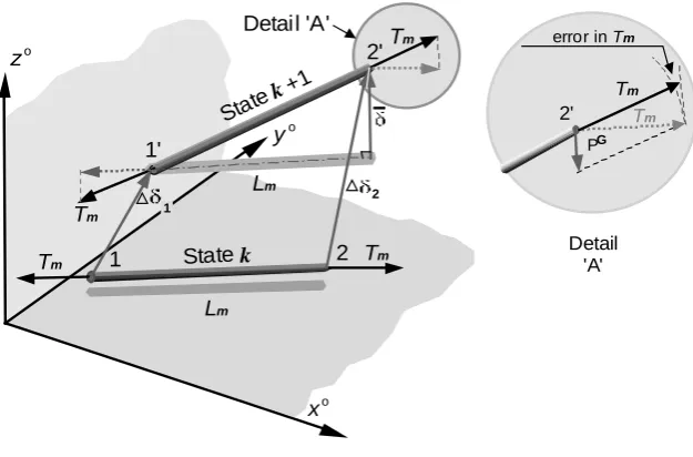
Figure 2 shows a member 1-2 displaced from state ‘k’ to state k+1’. It can be seen that
the incremental nodal displacement vector,
{ }
∆δj , may be replaced by a sum ofvectors parallel and perpendicular (orthogonal) to the member in state k.
z o
x o
Detail 'A'
State k
Lm
Lm
Tm
2
Tm 1
1
2'
1' y
o State
k+1
Tm
Detail 'A'
error in Tm
2'
P G Tm
Tm
Tm
[image:8.595.142.455.172.378.2]2
Fig. 2. Geometric forces in transient stiffness formulation
Hence
{ }
∆δj ={
∆δj,par} {
+ ∆δj,orth}
j =1, 2 (5)The magnitude of the parallel vector
{
∆δj,par}
is:{
}
{ }
{ }
jT par
,
j c δ
δ = ∆
∆ (6)
where
{ }
c is the vector of direction cosines (Fig. 3), corresponding to the iterative state 'k' .The components of vector
{
∆δj,par}
in global co-ordinates are:{
∆δj,par}
={ }{ }
c c T{ }
∆δj . (7)Now, the displacement vector orthogonal to the member is:
z z
y y
m
L x x
o 1 o 2
o 1 o 2
o 1 o 2
cos cos cos
− =
− =
− =
γ β α
m
L
m
L y o
x o o
z
1
β δ
α
2
(xo
2, yo2, zo2)
(xo
1, yo1, zo1)
xo 2
yo 2
zo 2
[image:9.595.192.399.77.221.2]Lm
Fig. 3. Geometric illustration of direction cosines
It can be seen from Fig. 2 that for small angles of rotation, the difference between the
orthogonal vectors of displacements at each end of the element can be taken as a
measure of rotation, denoted by δ. Hence,
{ }
δ ={
∆δ2,orth} {
− ∆δ1,orth}
=[
[ ]
I3 −{ }{ }
c cT]
{
{ } { }
∆δ2 − ∆δ1}
(9)The element carries the initial tension force, Tm. Provided the rotations are small, it
can be assumed that the components of force Tm parallel to the element in state k+1
do not differ significantly from Tm. Hence the only 'new' components of forces are perpendicular ones. As the direction cosines enter the stiffness matrix formulation,
and the calculation of stiffness lags one iteration behind, (eqn. (3)), these force
components are perpendicular to the direction of the element in state k, not k+1. As a
result, a degree of error is built into the formulation. The perpendicular force
components of Tm are the 'geometric’ forces,
{ }
PG , illustrated in Fig. 2.For the system of nodal forces to be in equilibrium, the moment about end '1'
generated by the initial tension force Tm on the lever arm δ must be balanced by the
moment due to the geometric force
{ }
Gδ K L δ T P G m m
G = =
, (10)
where m m G
L
T
K
=
, given as the ratio of pre-stress force to the current length of member,is known as the geometric stiffness.
Substituting for δ from eqn. (9) and using matrix notation, the geometric forces at
each end of the element are:
{ }
{ }
{ }
(
{ }{ }
)
(
{ }{ }
)
{ }{ }
(
)
(
{ }{ }
)
{ }
{ }
δ , K δ c c I c c I c c I c c I L T δ δ L T P j G j T T T T m m m m G = ∆ − − − − − − = − = 3 3 3 3 (11)The geometric stiffness defined in the above equation expresses a change in the nodal
force components due to the presence of pre-stress when there is a change in the
geometry of the structure during computation.
2.2 Evaluation of the method
2.2.1 The inclusion of elastic effects.
In some formulations 2,3,4,5 both the elastic and geometric effects are included in
form-finding calculations. Such an approach is not, in principle, necessary, as form-form-finding
calculations can apply to any type of material. Although the inclusion of the elastic
stiffness matrix has the advantage of increasing of the overall stiffness, which helps to
keep the increments of displacements
{ }
∆δj small, at the same time, it introduces significant complications, such as:• a need for control/monitoring of the values of the tension forces, which would
If not monitored, this situation could lead to a form-found configuration in which
safe loads are exceeded
• a necessity for adjustments of the unstrained cable lengths, in order maintain the
required tension levels (and prevent the problem stated above)
• a necessity for additional iterations, in order to restore static equilibrium after the
adjustments to unstrained lengths of cables.
2.2.2 Accuracy
The transient stiffness method is critically dependent on the assumption of small
displacements and rotations. Otherwise, large changes of geometry, which are
common in the initial stages of computational form-finding, would result in the nodal
forces and nodal displacements not being related to each other correctly. Potentially,
this could lead to either a lack of convergence of the solution, or a wrong solution.
The transient stiffness matrix requires numerous matrix manipulations, even for small
systems. For large systems, if matrix inversion is used, the solution may be prone to
divergence, or yield useless results, due to computational round-off errors,
exacerbated by ill-conditioning. A matrix is said to be ill-conditioned, if it contains
coefficients that are orders of magnitude greater (or smaller) than other coefficients.
The problems likely to arise in arithmetic operations on of ill-conditioned matrices
include 'swamping' the effects of small terms, or 'loss of significance' in the case of
small differences between large numbers containing too few figures to maintain
accuracy 6.
To mitigate round-off, techniques such as scaling of the stiffness matrix6,7 are
recommended, but they add to the computational effort. It is well-known 7, 8 that if
the size of the matrix is n x n, then the total number of arithmetic operations required
3. Force density
The force density method 9,10 was developed simultaneously with the transient
stiffness to facilitate the design of the Munich Olympic roofs. The method uses a
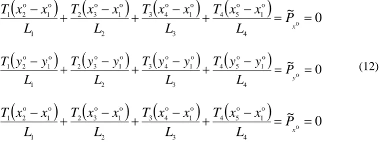
surface discretised as a system of branches. A simple branch of just four cables is
shown in Fig. 4. Nodes 2 to 5 represent boundary points with known co-ordinates,
expressed in the global xo, yo and zo system.
x o z o
y o
T 1
2
5 4
3 1
[image:12.595.91.475.548.694.2]T 2 T 3 T 4
Fig. 4. A branch of elements
The equations of equilibrium of forces at node 1 are obtained by resolving the tension
forces T1 - T4 into the global components, and summing up their respective contributions at the common node. Hence:
(
)
(
)
(
)
(
)
0
o 4 o 1 o 5 4 3 o 1 o 4 3 2 o 1 o 3 2 1 o 1 o 21
−
+
−
+
−
+
−
=
=
x
P
~
L
x
x
T
L
x
x
T
L
x
x
T
L
x
x
T
(
)
(
)
(
)
(
)
0 o 4 o 1 o 5 4 3 o 1 o 4 3 2 o 1 o 3 2 1 o 1 o 21 − + − + − + − = =
y P~ L y y T L y y T L y y T L y y
T (12)
(
)
(
)
(
)
(
)
0
o 4 o 1 o 5 4 3 o 1 o 4 3 2 o 1 o 3 2 1 o 1 o 21
−
+
−
+
−
+
−
=
=
x
P
~
L
x
x
T
L
x
x
T
L
x
x
T
L
x
x
T
In the above system of equations, the member lengths Lm, (m = 1,...4) are non-linear
unknown. By introducing constant values of tension coefficients, or force densities,
qm, defined as a ratio of member force to member length, viz., , m m m
L T
q = the system
of equations becomes linear, viz.,
(
2o 1o) (
2 3o 1o) (
3 4o 1o) (
4 5o 1o)
0
1
x
−
x
+
q
x
−
x
+
q
x
−
x
+
q
x
−
x
=
q
(
2o 1o) (
2 3o 1o) (
3 4o 1o) (
4 5o 1o)
0
1
y
−
y
+
q
y
−
y
+
q
y
−
y
+
q
y
−
y
=
q
(13)(
2o 1o) (
2 3o 1o) (
3 4o 1o) (
4 5o 1o)
0
1
z
−
z
+
q
z
−
z
+
q
z
−
z
+
q
z
−
z
=
q
With the qm values known, the co-ordinates of node 1 can now be found, as:
4 3 2 1 o 5 4 o 4 3 o 3 2 o 2 1 o 1 q q q q x q x q x q x q x + + + + + + = (14)
and similarly for the y1o, and z1o directions.
3.1 Matrix formulation
In a general case, for a member m with end nodes j and n, the length components Lmx, Lmy, and Lmz of the vector
{ }
L
m can be expressed using connectivity matrix [C]and their nodal co-ordinates as in:
[
]
[ ]
C{ }
Xx x x x L n j n j mx = − = − = o o o o 1 1
[
]
[ ]
C{ }
Yy y y y L n j n j my = − = − = o o o o 1
1 (15)
[
]
[ ]
C{ }
Zz z z z L n j n j mz = − = − = o o o o 1 1
In the case of the structure shown in Fig. 4, the projected lengths of members 1 to 4 in
− − − − = − − − − = o 1 o 5 o 1 o 4 o 1 o 3 o 1 o 2 5 o 4 o 3 o 2 o 1 4 3 2 1 1 0 0 0 1 0 1 0 0 1 0 0 1 0 1 0 0 0 1 1 x x x x x x x x x x x x x L L L L o x x x x
, (16)
where [C] is the connectivity matrix. In order to prevent the matrix becoming sparse,
and to facilitate computations, the following convention has been found helpful:
number the internal nodes first, and the boundary ones last.
Extending to y and z directions, the general form is
{ }
Lmx =[ ]
C{ }
X{ }
Lmy =[ ]{ }
C Y (17){ }
Lmz =[ ]
C{ }
ZThe x, y and z components of internal forces in cable members, given by, P~mx,
my
P~ ,P~mz, respectively can be expressed as a product of force densities, qm, and
projected member lengths, which, in matrix notation, are:
[ ]
Pmx[ ]
Q{ }
Lmx~ =
[ ]
Pmy[ ]
Q{ }
Lmy~ =
, (18)
[ ]
Pmz[ ]
Q{ }
Lmz~ =
where [Q] is the diagonal matrix of force densities,
[ ]
= 4 3 2 1 q . . . . q . . . . q . . . . q Q (19)At each node of the structure, the sum of the x, y and z components of the internal forces P~m in members connecting to the given node must balance the external load vector {P} applied to these nodes. Hence:
o
x mx
P
P
~
=
∑
o
y my P P~ =
∑ (20)
o
z mz
P
P
~
=
∑
Substituting for P~mx, P~my,P~mz from eqns. (18) and (17), and noting that the summation in eqn. (20) can be carried out by pre-multiplying the internal force components P~mx,
my
P~ , and P~mz by [C]T, leads to the matrix form :
[ ] [ ][ ]
{ }
{ }
xoT P X C Q C =
[ ] [ ][ ]
{ }
{ }
yoT
P Y C Q
C = (21)
[ ] [ ][ ]
{ }
{ }
zoT P Z C Q C =
Applying this result to the five-node, four-member structure shown in Fig. 4, gives,
for the x direction:
[ ] [ ][ ]
{ }
= − − − − − − − − = o 5 o 4 o 3 o 2 o 1 o 1 o 5 o 1 o 4 o 1 o 3 o 1 o 2 4 3 2 1 T 1 0 0 0 0 1 0 0 0 0 1 0 0 0 0 1 1 1 1 1 x x x x x P P P P P x x x x x x x x q . . . . q . . . . q . . . . q X C QIn the above system of equations, o 1x
P
is zero and the remaining forces are equal to the x-components of the reactions at the boundaries (nodes 2-5). Hence:[ ] [ ][ ]
{ }
= − − − − − − − − = o 5 o 4 o 3 o 2 o 1 o 5 o 1 o 4 o 1 o 3 o 1 o 2 4 3 2 1 4 3 2 1 0 0 0 0 0 0 0 0 0 0 0 0 0 x x x x T P P P P x x x x x x x x q q q q q q q q X C Q C (23)The equilibrium equations in the remaining y and z directions can be expanded in the
similar manner.
From eqn. (23) the x-co-ordinate of node 1 is:
4 3 2 1 o 5 4 o 4 3 o 3 2 o 2 1 o 1 q q q q x q x q x q x q x + + + + + + = ,
(confirming the earlier result), and the remaining external force components are given
as:
(
)
2 oo 1 o 2
1 x x Px
q − = ;
(
)
3 o o1 o 3
2 x x Px
q − = ;
(
)
o4 o 1 o 4
3 x x Px
q − = ;
(
)
5 o o1 o 5
4 x x Px
q − = (24)
3.2 Evaluation of the method
With boundary configurations known or assumed, the only other factor controlling the
shape of the structure is the value of force densities. This, theoretically, provides an
opportunity for generating an infinite number of network configurations. However,
such configurations may compromise the uniformity of the tension field i.e., they may
carry unacceptably high range of tension forces. It is clear that a constant value of
force density will not, in general, produce constant tensions, unless the calculated
lengths of the elements happen to be constant. From the practical point of view, the
results should produce a network with, ‘more or less’, equal forces in them, so that
load analysis stage). It has been found that a value of force density quoted as
producing reasonable results is 1 for all inner cables, and a value inversely
proportional to the cable length for boundary cables, when such cables have irregular
lengths 11,12.
In general, the system of linear equations given by the force density approach cannot
be solved directly, because of the size of the matrix. The limitations of the force
density method were realised quite early, and this has led to further developments, to
include additional constraints, such as the preservation of rectangular, or equidistant
meshes11. More recent additions include the facility to model minimal surface forms
by preserving a constant tension field13. In such cases, the formulation becomes a
non-linear force density method and requires additional iterative procedures to satisfy
the required condition. Some researchers14 advocate the use of surface minimisation
through least squares fit to arrive at a minimal surface solution. In the opinion of the
author, surface minimisation is not a robust criterion for convergence of the
solution15; it would require a very fine mesh of elements and the sum of their area
would be subject of a cumulative round off error.
4. Dynamic relaxation method
Unlike the previous two methods, dynamic relaxation does not rely on the global
stiffness matrix formulation for the solution of the system of non-linear equilibrium
equations. The algorithm uses a ‘lumped mass’ model, in which the mass of a
discretised continuum is assumed to be concentrated (lumped) at the nodes of the
surface. In the iterative scheme, the out-of-balance forces are relaxed, at each node in
turn, until they are close to zero. The solution follows a process in which static
time’. In essence, under the influence of loading (out-of-balance internal forces), a
system of lumped masses oscillates about the equilibrium position and eventually
comes to rest under the influence of damping. In its original form, the method makes
use of viscous damping, as described in the following section.
4.1 Dynamic relaxation method with viscous damping
The method is based on the equation of motion, which, for a discretised system is
given by:
[
]
ji ji ji jiji K M C
P = ∑ δ + δ + δ (25)
where
subscript ji refers to the jth node in the ith direction in a discretised system,
Pji is the vector of external loads,
[
∑ δK]
ji is the vector of internal loads, (with K representing nodal stiffness and δdisplacements and the summation applying to the connected nodes only),
ji ji,
δ
δ
, are the vectors of nodal accelerations and velocities, respectively,C is the coefficient of viscous damping Mji is the mass lumped to the nodes .
Introducing the nodal residual forces, Rji as the difference between the external and
internal force vectors, gives
[
]
jiji
ji P Kδ
R = − ∑ (26)
The above equation applies to the load analysis, which follows the form finding stage
and which includes elastic straining components in the formulated stiffness matrix,
external load acting on the inner nodes of the structure (whose configuration we are
trying to find), the residual forces are simply equal to the internal force vector, P~ji . Hence,
ji ji P
~
R = (27)
ji
P
~
is found from the resolution of the internal forces, Tm, at the nodes of thestructure.
Also, from eqn. (26)
ji ji ji
ji C R
M δ + δ = . (28)
Equation (28) states that the motion of a system is produced by the out-of-balance
forces. The condition of static equilibrium requires these forces to come to zero.
Equation (28) is approximated by centred finite differences in which the acceleration
term is represented by the variation of velocities over the time interval, ∆t, and the velocity term as an average over the same interval. Thus, with k denoting the time
interval at which variables are calculated, the residual forces at time increment k∆t are given by: 2 2 1 2 1 2 1 2
1 − + −
+ + + − = k ji k ji k ji k ji ji k ji C t M
R
δ
δ
∆
δ
δ
, (29)
which gives the recurrence equation for velocities:
2 2 2 2 1 2 1 C t M R C t M C t M ji k ji ji ji k ji k ji + + + − = − + ∆ ∆ ∆ δ
δ . (30)
The velocities are then used to predict displacements at time k+1:
t k ji k ji k
ji
δ
δ
∆
δ
21
1 +
The iterative process of arriving at static equilibrium consists of a repetitive use of
eqns. (30) and (31) until the residual forces are close to zero.
4.1.1 Stability and convergence of the iterative solution
The criterion for assured convergence 15,16,17, is given by
K M
t 2
Δ max = (32)
The time increment ∆t=1 is both convenient and the one that satisfies the limit for stability of the numerical solution. Thus, for ∆t=1, the mass at any node should be set to comply with eqn.(32), viz.,
2 2
Δ 2
ji ji ji
K K t
M = = (33)
4.1.2 Critical viscous damping coefficient
In an un-damped mode, the structure will oscillate about its position of equilibrium.
If N denotes the number of iterations required to complete one cycle of oscillations in
a fundamental mode, then the viscous damping coefficient, known as critical
damping, can be found from15:
C=4πmf , (34)
where f =1/N∆t, is the fundamental frequency of oscillations.
In order to obtain N, an additional computer run is necessary, with C set to zero. The
resulting un-damped oscillations of the structure are then used to calculate the value
Critical damping, which is based on the lowest natural frequency of the system, gives
the fastest convergence. If the damping coefficient is below this value, (the structure
is said to be ‘under-damped’) the solution may overshoot the static equilibrium of the
system, before settling down to convergence. This situation is preferred to the case of
an ‘over-damped’ solution, in which the convergence may proceed at a very slow
pace.
The requirement for a two-stage solution procedure is rather inconvenient. For this
reason, the method has been superseded by the dynamic relaxation technique with
kinetic damping.
4.2 Dynamic Relaxation method with kinetic damping 4.2.1 General
When the technique of kinetic damping is employed, the viscous damping coefficient
is taken as zero and the system of oscillating masses is brought to rest by following a
process of stopping the iterations whenever a peak in kinetic energy of the entire
system is detected. The computation is then re-started from the current configuration,
but with zero initial velocity15, 16. This process relies on the observation that, in simple
harmonic motion, maximum kinetic energy is achieved in a configuration that
corresponds to a minimum potential energy. A simple illustration of that is a motion
of a pendulum, which, once set in motion, eventually comes to rest in its position of
minimum potential energy. In the dynamic relaxation algorithm, the movement of the
structure is mapped by the successive iterations. The pendulum analogy shows that
stopping that movement (iterations) at the points of maximum kinetic energy is
equivalent to achieving a stable equilibrium position. However, because the
true overall equilibrium of the structure after the first kinetic energy peak. During the
next iterations, the velocities and the displacements accumulate, but in increments
decreasing in magnitude, as the residual forces become smaller with each iterative
step. This results in the peaks of kinetic energy gradually becoming less pronounced,
and eventually the whole system settling down to static equilibrium. The formulation
of the dynamic relaxation algorithm with kinetic damping is described below.
With the viscous damping coefficient equal to zero, and the time increment ∆t=1, equation (30) in centred finite difference form6, is:
−
=
+ −21 2 1 k ji k ji ji k ji
M
R
δ
δ
. (35)Implementing the numerical stability criterion given by eqn. (33) gives
−
=
+ −21 2 1
2
k ji k ji ji k jiK
R
δ
δ
Consequently, the recurrence equations for velocities and displacements are:
ji k ji k ji k ji K R 2 1 2 1 2 1 + = − +
δ
δ
. (36)and
1
2 1 1= + + ⋅
+ k
ji k ji k
ji
δ
δ
δ
. (37)As can be seen form the above, the method makes use of the nodal stiffness, Kji. The
stiffness needed here is the geometric stiffness, lumped at the nodes, viz.,
∑ = G m G ji K K
4.2.2 Iterative process
Equations (27), (36) and (37) form an iterative loop of the dynamic relaxation
algorithm with kinetic damping. At kinetic energy peak, velocities are set to zero and
the whole system is re-started from the current configuration. It can be deduced that
kinetic energy peak has occurred when the latest value of the kinetic energy is noted
to be smaller than that in the previous iteration. With the iterative process punctuated
by discrete time intervals, ∆t, the precise location of the point at which a maximum value of kinetic energy has occurred is not known, but can be estimated. It is
important to do so, in order to correct the displacements, as these would have been
calculated after a kinetic energy peak has occurred. The point of maximum kinetic
energy can be found by assuming that the trace of the kinetic energy curve represents
a quadratic variation with the number of iterations. If the time at which the kinetic
energy peak has occurred is denoted by tmax, and KE1, KE2, and KE3, denote three sequential energy levels at some point during iterations in which KE3 < KE2, it can be
shown that15
1 2 3
3 1 2
max
2 3 4
KE KE KE
KE KE KE
t
+ −
− −
−
= , (38)
and the corrected displacements at tmax are:
ji k ji )
k ( ji )
k (
ji corr ) k ( ji
K R
δ
)
β
(
δ
δ 1 2 2
1 1
1 − = + − + − −
+
, (39)
where
1 2 3
2 3
2KE KE KE
KE KE β
+ −
−
= . (40)
When kinetic energy peak is detected, the displacements are calculated according to
4.3 Evaluation of the method
The main advantage of the method is the small number of arithmetic operations that
need to be carried out at any one time, since the computations are concerned with one
node in turn, rather than all nodes simultaneously. Such an approach minimises
computational round-off errors, and contributes to stability and accuracy of the
numerical solution. It has been shown15,18 that the method is more efficient than the
transient stiffness solution.
Experience has shown15,16 that the numerical stability criterion for the dynamic
relaxation method is robust, provided the largest direct stiffness of the connecting
elements is used to ensure as small as possible size of the iterative step. The criterion
is based on the assumption of constant mass and stiffness. A derivation of a stability
criterion based on variable lumped mass and stiffness would be an advantage, and this
subject merits further study. The method is stable and capable of providing solutions
to highly non-linear problems, even if the criteria of constant mass and stiffness are
not met. However, to ensure fast convergence and stability of iterations, it is
recommended that the difference in nodal stiffness throughout the structure is kept
small. This can be achieved by an appropriate surface discretisation, involving the
same, or similar, number of elements connecting to each node of the structure.
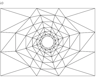
4.4 Surface discretisation and accuracy of modelling 4.4.1 Line elements
Surface discretisation by means of line elements is equivalent to replacing the surface
by a cable net. Such a net, when used to model stable minimal surfaces (soap-films)
has all its elements in constant tension and the elements following geodesic paths15.
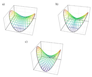
with more pronounced curvatures, the cables have a tendency to cluster in the areas of
high curvature and become sparse elsewhere. This phenomenon is illustrated in Fig.
5, which shows a saddle shaped surface modelled with cable elements of constant
[image:25.595.113.465.173.467.2]tension.
Fig. 5. Line element representation of a saddle-shaped surface modelled by constant tension cables
There are 15 cables in each direction and the boundary of the structure projects as a
circle of 6 unit’s radius. The aspect ratio of height to radius is 0.528 for case (a) and
0.846 for cases (b) and (c). It can be seen that with the rising aspect ratio, the cables
start to cluster in the area of high curvature (case (b)). Improvements in the final
surface definition can be made by carefully selecting the location of the end points, so
that after form-finding the cables slip into their equilibrium position while
maintaining a reasonably uniform spacing. This is illustrated in case (c). c)
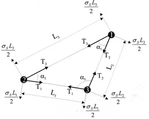
4.4.2 Triangular elements
The most common type of surface element used in conjunction with dynamic
[image:26.595.201.442.165.357.2]relaxation method is a triangular, or triple-force element, shown in Fig. 6.
Fig. 6. Triangular, ‘triple-force’ element
The formula:
i i s i
L T
α σ
tan 2
=
represents a transformation of the element surface stress into a discrete set of forces,
Ti, acting in the sides of the element. Depending on the value of the enclosed angle α,
the element side forces can be either positive, or negative. They are resolved into x, y
and z components at the nodes and included directly in the calculation of residual forces within the dynamic relaxation algorithm. However, caution is needed, as cases
of ill-conditioning can arise: when the angle α tends to zero, the forces tend to
infinity. The problem can be resolved by a sensible discretisation of the surface that
4.4.3 Alternative methods of surface discretisation
Alternative types of surface discretisations have been proposed for use with novel,
non-finite element approaches 19,20. The first one19, which applies to constant tension
membranes, makes use of a triangular mesh of points. The resultant forces at the
vertices of the triangle are calculated directly from the surface tension, without the
need for construction of equivalent plane stress finite elements. These forces are
independent of the shape of the triangular mesh. The other type of surface
discretisation20, which also applies to constant tension membranes, but can be
adapted to more general cases, makes use of the Laplace-young equation and cubic
spline fitting to give a full, piecewise, analytical description of the surface. This
approach represents a significant development in surface discretisation, as it produces
smooth surfaces with known curvatures that can be used readily to calculate geodesic
curves. Geodesics, combined with the knowledge of surface curvatures, facilitate the
development of cutting patterns. Also, the spline solution is much closer to the actual
surface than a polyhedral surface of elements of the same mesh size21 .
4.4.4 Mesh control
It is possible to find a shape of a tensioned surface by constraining the x, y
movements of the nodes of the initial mesh during form-finding and ensuring
equilibrium in z-direction only16. This approach was thought to assist with the
generation of smooth mesh lines at the end of form-finding so that they could be used
for patterning. The idea, however, is fundamentally flawed, because the mesh lines
intended to represent seam lines at the patterning stage should correspond to ‘strings’
of constant tension, lying on the surface and following geodesics15. These strings
Fig. 7. (a) Elevation of the form-found surface, (b) plan view of the surface obtained with mesh control, (c) plan view of the fully equilibrated surface.
(a)
(b)
[image:28.595.110.430.451.707.2]The chosen example is a membrane, which resembles a part of a canopy for the Tête
Defence Cube in Paris. The membrane is discretised using triangular elements, as
shown. The plan area of the membrane is 5 m by 7 m. The boundaries along the
shorter, x- dimension are fully fixed, while the two boundaries along the y dimension
are fixed only in the x and y directions. The central boundary, which is circular on plan, has a height of 0.9 m. The membrane has a constant value of prestress, equal to
5 kN/m. The value of the residual force used as a stopping criterion for the iterations
was 0.01 kN (a value lower than that showed no significant change in the solution).
The results from form-finding (Fig. 7 (a), (b, and (c) show that mesh control produces
the same elevation profile as the unconstrained mesh method. However, the
differences lie in the plan views, from which it can be seen that large displacements
would have taken place, if the x-y movements of the nodes were not suppressed. The
surface obtained using mesh control is not in full static equilibrium, as shown by the
results given in Table 1. They illustrate that very large residual forces still exist in the
x and y directions (several orders of magnitude higher than the prescribed maximum residual force of 0.01 kN) particularly at the nodes along the lines 2-6 and 9-10.
These findings are consistent with the report22 describing form-finding and patterning
of a Papal canopy in Phoenix Park, Dublin. The canopy resembled the membrane
shape analysed here, but possessed only one axis of symmetry. Mesh control was
applied during form-finding to preserve the radial lines as seam lines in the cutting
pattern of the membrane. This led to a very uneven stress distribution in the surface,
manifesting itself in wrinkling around the neck of the structure, which required a
5. Closing remarks
The paper describes three most commonly used computational form-finding methods,
which have been implemented in commercial software world wide.
The transient stiffness method exploits load-displacement relationship, which is
assumed to be linear throughout. For this to be true, the incremental displacements
have to be very small. In the case of an ill-conditioned stiffness matrix, steps need to
be taken to remedy the situation, in order to obtain an accurate solution.
The force density method, in its original formulation, is just a tool for generating
equilibrated shapes of structures that have the feature of a non-uniform tension field.
Additional iterations are required to satisfy the condition of constant tension, as
observed in ideal tension structures, such as soap-films. The use of soap-film analogy
in form-finding of fabric structures is strongly recommended15, as it leads to optimal
solutions in the form of minimal surface membranes, with a uniform tension field
under a permanent load condition, i.e., the pre-tension. This view is reflected in the
general recommendation given in the European Design Guide for Tensile Surface
Structures23. To start, section 8.2 of the Guide contains a somewhat indefinite
statement saying that any form-finding method is acceptable, provided it ensures
that… “the resulting surface shape is capable of withstanding the applied loading,
while satisfying the constraints imposed by the architectural specification”… While this appears to give priority to architectural requirements, the statements that follow
acknowledge the advantages of using the soap-film analogy. These include: (i) a
reduced likelihood of on/off slackening of the fabric under buffeting wind loads, with,
consequently, less fatigue of the yarns and their constituent fibres, and (ii) a smaller
deformation of the surface due to a change in the warp/weft stress ratio, which is
differentially stressed fabric will creep, over a period of time, towards a form that has
a uniform stress distribution.
In the UK, the preferred form-finding method is dynamic relaxation24. It is viewed as
extremely efficient, robust and accurate. Further, it has an attractive physical
interpretation, which aids a good understanding of the solution process.
Acknowledgement. The author wishes to thank her research fellow, J.S. Brew, for
supplying Figure 5.
References
1. FORSTER B. Cable and membrane roofs - a historical survey. Structural Engineering Review, 1994, 6, No 3-4, 145-174.
2. ARGYRIS J. H. and SCHARPF D. W. Large deflection analysis of prestressed networks. Journal ASCE, Structural Division, ST3, 1972, pp 633-654.
3. ARGYRIS J. H., ANGELOPOULOS T. and BICHAT B. A general method for the shape finding of lightweight tension structures. Computer Methods in Applied Mechanics and Engineering, 1974, Vol. 3, pp 135-149.
4. LEONARD J. W. Tension structures. Behaviour and analysis. McGraw Hill Book Company, 1985.
5. MEEK J. L. Computer methods in structural analysis. E&FN Spon, 1991.
6. CHAPRA S. C. and CANALE R. P. Numerical methods for engineers. McGraw Hill, 1985, 2nd edn.
7. WILKINSON J. H. and REINSCH C. Linear algebra. Handbook for automatic computation. Springer, Berlin , 1971.
8. FOX L. An introduction to numerical linear algebra. Clarendon Press, Oxford, 1964.
9. LINKWITZ K. and. SCHECK H. J. Einige bemerkungen zur berechnung von vorgespannten seilnetzkonstruktionen. Ingenieur - Archiv. 1971, 40, 145-158.
11. SCHECK H. J. The Force density method for form-finding and computation of general networks. Computer Methods in Applied Mechanics and Engineering, 1974, 3, 115-134.
12. LINKWITZ K. About formfinding of double-curved structures. Engineering Structures, 1999, 21, 709–718.
13. SANCHES J. et al. A multi-step force-density method and surface fitting approach for the preliminary shape design of tensile structures. Engineering Structures, 2007, 8, 1966-1976.
14. GRÜNDIG L. Minimal surfaces for finding forms of structural membranes. Computers & Structures, 1988, 30, 679-683.
15. LEWIS W. J. Tension structures. Form and behaviour. Thomas Telford 2003.
16. BARNES M. R. Form and stress engineering of tension structures. Structural Engineering Review, 1994, 6, No. 3-4, 175-202.
17. BREW J. S. and BROTTON D. M. Non-linear structural analysis by dynamic relaxation. International Journal of Numerical Methods in Engineering, 1971, 3, 463-483.
18. LEWIS W. J. The efficiency of numerical methods for the analysis of prestressed nets and pin-jointed frame structures. Computers & Structures, 1989, 33, no. 3, 791-800.
19. BREW J.S. and LEWIS W.J. Computational form-finding of tension membrane structures - non-finite element approaches: Part 2. Triangular Mesh Discretisation and Control of Mesh Distortion in Modelling Minimal Surface Membranes. International Journal for Numerical Methods in Engineering, 2003, 56, 669-684.
20. BREW J.S. and LEWIS W.J. Computational form-finding of tension membrane structures - non-finite element approaches: Part 1. Use of cubic splines in finding minimal surface membranes. International Journal for Numerical Methods in Engineering, 2003, 56, 651-668.
21. BREW J.S. and LEWIS W.J. Computational form-finding of tension membrane structures - non-finite element approaches: Part 3. Comparison of mesh constraint methods. International Journal for Numerical Methods in Engineering, 2003, 56, 685-697.
22. DAY A. Form-finding, Control and modification for tension structures. The Arup Journal, 1980, 19-20.
23. FORSTER B. and MOLLAERT M. European design guide for surface tensile structures. Tensinet 2004.