Comparison between Results of Different Methods of
Determination of Water Surface Elevation in Tidal Rivers and
Determination of the Best Method
Arash Adib
*, Ali Banetamem, Abbas Navaseri
1Department of Civil Engineering, Engineering Faculty, Shahid Chamran University of Ahvaz, Iran
Received 26 February 2017; accepted 6 March 2017, available online 6 March 2017
1. Introduction
Effect of tidal surges on tidal rivers is a very complex problemin hydraulic routing in tidalrivers. Combination of flood and tidal surge can become a potential damage source for cities, farms, factories and people of around of tidal rivers. Because of determination of maximum water surface elevation in different sections of tidal rivers is a very important; a suitable method must be developed. Two governing factors in tidal rivers have different sources. Fluvial flows depend on hydrological conditions and characteristics of watershed (intensity and regime of precipitation, vegetation cover and type of soil, slope of river and slope of watershed, concentration time and etc). Tidal surges have two sources; periodic sources and non-periodic sources. Effects of gravity of the moon and the sun are periodic sources. Effects of shallow water, wave reflection and marine hurricanes are non-periodic sources. Because the sources of fluvial flows and tidal surges are different, they had to be combined by a suitable method. Analytic methods and numerical models can not be applied alone for hydraulic routing in tidal rivers. Stochastic approach must be considered too.
Some researchers used analytic methods for separation tidal flow and fluvial flow. A researcher studied the effects of the increase in discharge of rivers and effects of the different kinds of tides (neap or spring tide) on amplitude of tide and travel time of tide to the upstream of river. He used a perturbation method to determine variations of water surface elevation in tidal rivers by tidal flows. He supposed that discharge of a
river was constant and that tidal flow was unsteady. Based on results of his research, the increase of discharge decreases the amplitude of tide and increases the travel time of tide to upstream. In neap tide, the amplitude of tide decreases and travel time of tide to upstream increases. In spring tide, the amplitude of tide increases and travel time of tide to upstream decreases [1]. Also other researchers used an unstable time –dependent interaction method and a stable quasi-steady interaction method to solve the equation of the perturbation method in Chao Phraya River. They observed that the quasi- steady interaction method has more accurate results than the unstable time- dependent interaction method [2].
By progressing of computer science and developing numerical models, some researchers utilize numerical models for hydraulic routing in tidal rivers. A researcher utilized characteristics method [3] and some used from upwind scheme and finite volume method for solving the shallow water equations in tidal rivers [4]. A number of scientists studied the joint probability approach in river flood and tidal surge interaction [5 to 7]. They developed an equation for combination coefficient but no stochastic method was utilized [7] while others dealt with the same problem from a different perspective [5, 6]. Researchers developed three Back-Propagation Neural Network models in order to improve the accuracy of prediction and supplement of tidal records: (1) Difference Neural Network model (DNN) for the supplementing of tidal record; (2) Minus-Mean-Value Neural Network model (MMVNN) for the corresponding prediction between
Abstract: Fluvial flows in the upstream of tidal rivers and tidal surges in the downstream of them are governing factors in tidal rivers. Hydraulic routing is a very difficult problem in tidal rivers. In this research, three methods are developed for determination of water surface elevation in tidal rivers. Results of these methods are compared to results of conventional method. These methods are applied for the Karun River. Selected reach locates between Ahvaz in the upstream and there branches junction of Khoramshar in the downstream. At the first, a numerical model is developed and envelopes of curves are extracted by results of this model. Then, structural regression relations which are governing on envelopes of curves aredetermined. In the other hand, a neural network is trained by results of numerical model. At the end, results of envelopes of curves method, structural regression relations method and neural network method are compared. Results of different methods show that calculated water surface elevation by conventional method is very conservative. For 100 years return period, calculated water surface elevation by conventional method is almost 10 cm more than calculated water surface elevations by other methods.
tidal gauge stations; (3) Weather-Data-based Neural Networks model (WDNN) for set up and set down. The results show that the above models perform well in the prediction of tidal level or supplement of tidal record including strong meteorological effects [8].
Two researchers applied different ANNs (multilayer Forward (FF), Cascade-Forward (CFF), Feed-Forward Time-Delay (FFTD), Radial Basis Function (RBF), Generalized Regression (GR) neural networks and Multiple Linear regression (MLR) methods) for tidal prediction model. The input data set used in the study, contains tide gauge data obtained at the town of Burgas, located at the western Bulgarian Black Sea coast for the period 1990–2003.The ANNs offer an effective approach to correlate the nonlinear relationship between an input and output of the sea levels by recognizing the historic patterns between them. The obtained results indicate that the artificial neural technique is suitable for short and long-term forecasts of the sea level parameters [9].Also scientists applied a preliminary empirical orthogonal function (EOF) analysis in order to compress the spatial variability into a few eigenmodes, so that GA could be applied to the time series of the dominant principal components (PC). The multivariate version of GA has been used to carry out the forecast using a few tidal levels at the boundary of the domain of study as inputs. The performance of this combined technique has been found to be quite satisfactory [10].
Iranian researchers used of artificial neural network (ANN) and genetic algorithm (GA) method for determining tide velocity, ebb velocity and variation of water surface elevation by tidal flow. Inputs of ANN were discharge of fluvial flow, domain of tidal cycle and distance from the mouth of tidal river. They concluded that results of trained ANN by GA are more accurate than results of ANN. GA increases regression coefficient between output of ANN and desired output from 1% to 8% also decreases MSE extremely (43% to 85%) [11]. Also they applied two perceptron artificial neural networks and Levenberg–Marquardt training method for determination of suspended sediment concentration. They applied GA for increasing regression coefficient and decreasing MSE. Inputs of first network were distance from upstream of river, flood return period, and tide return period. Inputs of second network were distance from upstream of river, flood discharge, and ebb height [12]. They applied artificial neural network (ANN) and genetic algorithm (GA) methods for calculation salinity concentrations in tidal rivers too. Inputs of network were distance from upstream of river, flood discharge, and tidal height. GA method decreases the mean of square error (MSE) 66.4% and increases efficiency coefficient 3.66% [13].
Researchers developed a three-dimensional salinity and fecal coli form transport model and incorporated into a hydrodynamic model. Their case study was the tidal Danshuei River estuarine system of northern Taiwan. The model was applied to investigate the effects of upstream freshwater discharge variation and salinity and fecal coli form loading reduction on the contamination distributions
in the tidal estuarine system. The qualitative and quantitative analyses clearly revealed that low freshwater discharge resulted in higher salinity and fecal coli form concentration [14]. Other researchers investigate how salinity changes with abrupt increases and decreases in river discharge around the Yellow River mouth [15].
Two researchers established a two-dimensional horizontal (2DH) numerical model of flow. They applied the Galerkin finite element method (FEM). The software Easy Mesh is used to triangulate the modeled planar domain. The two-step Lax–Wendroff scheme is used for integrating the equations in order to avoid the nonlinear iterative calculation. This two-dimensional horizontal finite element model was found to be well suited to the complexities of the North Passage of the partially-mixed Changjiang River estuary [16]. A scientist studied past researches about seawater intrusion management problem of coastal aquifers and tidal rivers. He considered effective factors on this problem (for example fresh water discharge, pumping rate, seawater volume into the aquifer and river, etc.). He illustrated that optimization methods can be classified to five categories: linear programming, nonlinear programming, genetic algorithms, artificial neural networks, and multi-objective optimization models [17]. In this research several methods are applied for determination of water surface elevation in tidal rivers while other researches only considered a method for determination of characteristics of tidal rivers.
2. Materials and Methods
2.1 Conventional Method
In conventional method, it is assumed that flood and tidal surge are two independent phenomena. If two phenomena are independent, probability of their intersection will become multiplication of their probabilities.
P (A∩B) = P (A)*P (B) (1) T (A∩B) = T (A)*T (B) (2)
where T is return period (year). Therefore conventional method considered two states for return period of intersection flood and tidal surge. These states are:
1. Flood with 1 year return period and tidal surge with N years return period.
2. Flood with N years return period and tidal surge with 1 year return period
N is return period of design flood. This method does not consider other states (for example flood with N/2 years return period and tidal surge with 2 years return period that multiplication of them is N). Because this method considers extremely events (flood and tidal surge with N years return period), results of this method are conservative. For reaching to suitable results, three methods are developed
.
2.2 Numerical Model
At the first, a numerical model was developed. This model makes used to Priessman method for solution Saint Venant equations. This model gets different boundary conditions and it is run for them contemporaneous. Model compares results of different boundary conditions and shows maximum water surface elevation for each section and each time step. The Saint Venant equations are the governing relations of the model and the Preissman method, a four point finite differences method, is applied for solution procedure.
q t A x Q (3) 0 2 2 ) ( 2 2 2 2 1 1 3 4 2 2 0 2 x C qv g v g v L C R A n Q Q S x h gA A Q x t Q
(4)where αi, αi+1 are correction coefficients for kinematics energy in sections i, i+1. β is momentum correction coefficient and A is cross sectional area (m2). CC is energy loss coefficient due to expansion or contraction of sections and g is gravitational acceleration (m/s2). H is water surface elevation (m) and L is distance between consecutive sections (m). n is Manning’s coefficient. Q is discharge (CMS) and q is discharge of lateral inflow per unit width of main channel (m2/s). R is hydraulic radius (m) and S0 is slope of the bottom of the channel. Vi, Vi+1 are flow velocities in sections i, i+1 and vx is component of velocity of lateral inflow that is parallel to the direction of main channel (m/s).
Equation (3) is the continuity equation and equation (4) is the momentum equation. Spatial and temporal discretization are made as follows based on the Preissman method:
t
f
f
f
f
t
f
ikk i k i k i
2
)
(
)
(
1 1 1 1 (5)x
f
f
f
f
x
f
ikk i k i k i
(
)
(
1
)(
1)
1 1 1
(6))
)(
1
(
2
1
)
(
2
1
1 1 1 1 k i k i k i ki
f
f
f
f
f
(7)f represents Q, A and h in equations (5) and (6) and represents V and R in equation (7).
is a weight factor.Different values of
are used for different methods (0for explicit forward method, 1 for fully implicit backward method and 0.5 for Crank-Nicolson method).
Manning’s equation has been used to determine the friction slope which has been assumed to be equal in the left bank, the right bank and the main channel in each section. Equivalent Manning’s coefficient is calculated by Horton-Einstein equation: 3 / 2 2 / 3
i i i ep
n
p
n
(8)where ni is Manning's coefficient in each part, ne is equivalent Manning's coefficient for cross section and pi is wetted perimeter in each part (m). The geometric part of model was developed using the trapezium method while available models make use of regression relation between depth of water and area, wetted perimeter and hydraulic radius. The trapezium method is found to be more exact. For considering of effects of bridges, culverts and other hydraulic structures, CC (energy loss coefficient) must be changed.
2.3 Envelopes of Curves Method
For producing envelopes of curves, different flood hydrographs in upstream boundary and different stage hydrographs in downstream boundary are exerted to numerical model. Then a number of levels are considered in different sections. Stages of downstream boundary and discharges of upstream boundary which produce considered levels are distinguished on stage of downstream boundary- discharge of upstream boundary graph. A curve which connects these points is envelopes of curve of considered level. Envelopes of curves are produced by different combinations of boundary conditions and they show average of results of different combinations which produce this envelope of curve. Results of envelopes of curves method are more accurate than conventional method because this method considers more combination of discharges of flood and stages of tidal surges. For using of envelopes of curves, peak of flood hydrograph and maximum tidal height of each combination are introduced to envelopes of curves graph of considered section and water surface elevation is determined for this combination. Water surface elevations of different combinations which produce combined return period are compared. Then maximum of them are selected.
2.4 Structural Regression Relations Method
Components of this relation are return periods of flood and tidal surges and distance from mouth of tidal river. Different forms of regression relations are considered (for example linear, logarithmic, exponential and etc). The best form of regression relations determine by least square error method.
This relation shows maximum water surface elevations of different sections for each design flood and combination which produces maximum water surface elevation for each section. Results of this method is more accurate than them of envelopes of curves method because this method considers combinations which combined return period of them is equal to return period of design flood while envelopes of curves method considers different combinations. Because combinations with return periods greater than return period of design flood increase water surface elevation in different sections, results of envelopes of curves method are higher than them of structural regression relations method.
2.5 Neural Network Method
Neural network method needs to very much data. Because of shortage of observed data, for training of a neural network using of not only observed data but also results of numerical model is necessary. After training of network, the best topology of network is distinguished. In this research, Nero solutions software is applied for neural network method. The arrival inputs to neural network are return periods of floods and tidal surges and distance from mouth of river. Other researchers introduce discharge of flood to neural network alone while two factors are governing on tidal rivers.
Learning rules in ANN are two types. In supervised learning, the learning is done on the bases of direct comparison between the output of the network and known correct answers (or target patterns). This is sometimes called learning with a teacher. The neural network is “trained” by repeatedly presenting examples of the inputs and desired outputs. As each example is entered into the network, the difference between the actual output of the network and the desired output is used to modify the weights for each interconnection. Training of the network (or equivalently, changing the values of interconnection weights) continuous until the actual output of all training examples matches the desired outputs to within some specified tolerance. When this is achieved, the neural network is said to be “trained” and is ready to accept new inputs to predict the outputs.
In unsupervised learning, a learning procedure in which the network is presented only a set of input patterns. The network adapts itself according to the statistical associations in the input patterns. The only available information is in the correlation of the input data or signals. The most important components in ANN are nodes. Nodes locate in layers. An ANN has three type layers. Input layer which receive input from external sources, compute their activation level, calculate their output as a function of activation level, and transmit this output to the rest of the network.
Output layer which receive input from the rest of the network, compute and broadcast their output to the external receivers. Hidden layers which only receive input from, and broadcast their computed output to, units within the network. For computation of output, each node receives a set of input from its neighbors (i.e. those processing units to which it is connected). There is a weight parameter assigned to each input value. Using input values and their weights, an activation level for each node is computed. This stage is called "activation propagation mechanism" which is usually a weighted sum of incoming values and a bias term (or threshold). The activation level is fed through an activation function and results in the output value of the node. Finally, this output is sent to the other nodes.
In general terms, larger number of nodes in the hidden layer(s) and increase in the number of hidden layers enable the network to learn more complex problems and better to represent the training data, but the training time will be increased and it may reduces the generalization capacity of the network. It means if the nodes in the hidden layer(s) are less than a special range, the network will not be able to solve complex problems, and if they are too high, the network may just represent the training data and its generalization capacity will be decreased. Therefore the number of hidden layers and the number of nodes that they contain, are important parameters that should be defined by user and are usually problem dependent.
The network topology (i.e. the number of layers, the number of nodes and their inter-connectivity), the rules of learning and functions of output and activation are all variable in a neural network and lead to a wide variety of network types. There are basically two main classes of networks: Feed forward networks, in which the nodes in the network are grouped into layers and communications are restricted to occur only between layers and in a forward direction, no lateral, self or back connections are allowed. Examples are: the Perceptron, Feed forward back-propagation and Radial basis function networks. Feed forward networks are suitable networks for engineering problems. Other networks in which the links can form arbitrary topologies (i.e. feed backward, recurrent, self-connection are involved). Examples are: Recurrent back-propagation network, Hopofield network, etc.
2.6 The Karun River
days. Floods that occur in March and April have long durations (more than ten days) and low peak flows (less than 2000 CMS). These floods are developed by rainfall and snowmelt. Tidal surges are diurnal in the mouth of the Karun River. The highest tidal surges occur in June and July. The governing stochastic distribution on annual maximum discharges is a log Pearson III distribution in the hydrometric station of Ahvaz. For different return periods, discharges of peak flow are shown in Table 1.
Table 1 Peak discharges of flood hydrograph for different return periods in the hydrometric station of Ahvaz
Return period (year) Peak discharge of flood (CMS)
1 2507
2 2802
5 3961
10 4606
20 5142
25 5297
50 5735
100 6118
The governing stochastic distribution on annual maximum tidal elevation is a Gumbel distribution in the three branches junction of Khoramshar. These data were prepared from Khuzestan Water & Power Authority (KWPA). In this research, used hourly water surface elevations were measured from 1965 to 2015. Annual maximum water surface elevations (50 data) were extracted from this time series. For different return periods, tidal elevations are shown in Table 2.
Table 2 Tidal elevations for different return periods in three branches junction of Khoramshar
Return period (year) Tidal elevation (m)
1 3.09
2 3.18
5 3.35
10 3.46
20 3.56
25 3.6
50 3.7
100 3.8
Fig. 2 Indicator flood hydrograph in upstream
Tidal limit locates between three branches junction of Khoramshar and 140 Km from Ahwaz in the Karun River.
Fig. 1 Map of the Karun River in Iran
Fig. 3 Indicator tidal height cycle in downstream
3. Results
3.1 Results of Envelopes of Curves Method
Envelopes of curves are shown for 180 Km distance from Ahvaz and Salmanieh Station in 159 Km distance from Ahvaz (Figs. 4 & 5).
Fig. 4 Envelopes of curves for Salmanieh Station
Fig. 4 Envelopes of curves for Salmanieh Station
Fig. 5 Envelopes of curves for 180 Km distance from Ahvaz
Envelopes of curves at 180 Km from the Ahvaz show that tidal surges are governing on this part of the Karun River. In this section, envelopes of curves are vertical in spite of the fact that the discharge is high. Envelopes of curves at Salmanieh Station show floods are governing on this part of Karun River. In this section, envelopes of curves are horizontal in spite of the fact that tidal height is high.
3.2
Results
of
Structural
Regression
Relations Method
In this research based on interaction between tidal surges and floods, water surface elevations were determined in different sections of tidal river. For determination of interactive return period, return period of flood and tidal surges must be considered. On the other hand, importance of flood or tidal surge at each point of river depends to distance of this point from the mouth of tidal river.
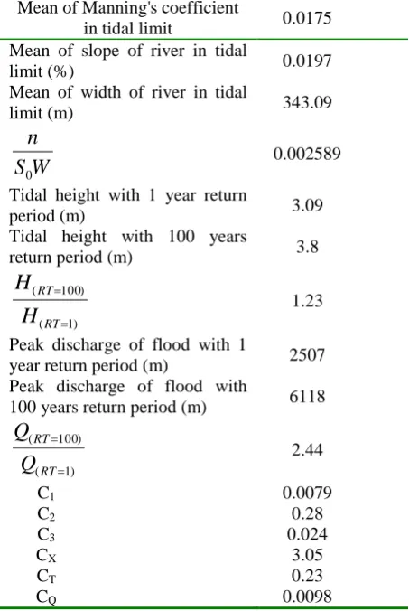
Therefore three coefficients are considered in structural regression relation. These coefficients are multiplied in distance from mouth of tidal river (C1), return period of tidal surge (C2) and return period of flood (C3). (C1) concerns to mean of Manning's coefficient, mean of slope and mean width of river in tidal limit of tidal river. (C2) concerns to relation between values of tidal heights with return periods 1 year and 100 years. (C3) concerns to relation between values of peak discharges of floods with return periods 1 year and 100 years. After testing of different regression relations by least square method, below regression relation is selected for the Karun River.
)
)
(
(
C
1X
C
2Ln
RT
C
3RQ
Exp
H
(9)W
S
n
C
C
X0
1
(10)) 1 (
) 100 ( 2
RT RT T
H
H
C
C
(11)) 1 (
) 100 ( 3
RQ RQ Q
Q
Q
C
C
(12)where: H is water surface elevation (m),
H
(RT1) is tidal height with 1 year return period in mouth of river (m),) 100 (RT
H
is tidal height with 100 years return period in mouth of river (m), n is mean Manning's coefficient intidal limit,
Q
(RQ1) is peak discharge of flood with 1 yearreturn period (CMS),
Q
(RQ100) is peak discharge of flood with 100 years return period (CMS), RQ is return period of flood (year), RT is return period of tidal surge (year), S0 is mean slope of river in tidal limit (%), W is mean width of river in tidal limit (m) and X is distance from mouth of river (Km). The values of these parameters and coefficients are shown in Table 3 for the Karun River. Because tidal surges are governing on tidal rivers in tidal limit of them, the most important coefficient is C2 which is concern to return period of tidal surges.3.3 Results of Neural Network Method
Nero solutions software tests different artificial neural networks. These networks have different structures. At the end, software selects the best network. Neural network method can get different combination of tidal surges and floods. Neural network method shows accuracy of results of structural regression relations method too. In this research, software selects a multilayer perceptron network. This network is a feed forward network and makes used to back propagation (B.P) learning algorithm. This learning algorithm compares outputs of network and desired outputs by least square method. Then, this learning algorithm sends information of error to nodes of network and training of network
4.6
4.4
4.2 4.0
3.8
440 0 490 0 540 0 590 0 640 0
3 3.2 3.4 3.6 3.8 4 4.2 Tidal height in 3 branches junction of Khoramshar
(m)
Dis
ch
ar
g
e
in
Ah
v
az
(
C
MS)
3.7 3.8 3.6
3.5 3.4
3.3
3.2
5000 5200 5400 5600 5800 6000 6200
3 3.2 3.4 3.6 3.8 4
Tidal height in 3 branches junction of Khoramshar (m)
Dis
ch
ar
g
e
in
Ah
v
az
(
C
continues. At the end, error of network reaches to a suitable value.
Because return period of flood, return period of tidal surge and distance from mouth of river are inputs of network, arrival layer of network has three nodes. Output of network is water surface elevation and output layer of network has a node. This network has two middle layers and each middle layer has three nodes. Activation function is hyperbolic tangent function in this network. Output layer makes used to bias function and adds bias to weight of connections. Learning algorithm converts bias and weights of connections and optimum values of bias and weights of connections are calculated. The momentum constant, error tolerance and learning rate of selected ANN are 0.6, 0.1 and 0.1 respectively.
441 training pairs (return period of tide and return period flood) were introduced to ANN. Return periods of these pairs are 0.01, 0.02, 0.025, 0.04, 0.05, 0.1, 0.2, 0.25, 0.4, 0.5, 1, 2, 2.5, 4, 5, 10, 20, 25, 40, 50 and 100. 80 percent of training pairs made used to training of ANN and 20 percent of them made used to validation of ANN. Network is trained 3000 times. Results of regression relation method and results of neural network method are compared in 180 Km from Ahvaz. This comparison is shown in Figs. 6 & 7.
Table 3 Values of parameters and coefficients of structural regression relations method for the Karun River
Mean of Manning's coefficient
in tidal limit 0.0175 Mean of slope of river in tidal
limit (%) 0.0197
Mean of width of river in tidal
limit (m) 343.09
W
S
n
0
0.002589
Tidal height with 1 year return
period (m) 3.09
Tidal height with 100 years
return period (m) 3.8
) 1 (
) 100 (
RT RT
H
H
1.23
Peak discharge of flood with 1
year return period (m) 2507 Peak discharge of flood with
100 years return period (m) 6118
) 1 (
) 100 (
RT RT
Q
Q
2.44
1
C 0.0079
2
C 0.28
3
C 0.024
X
C 3.05
T
C 0.23
Q
C 0.0098
Fig. 6 Comparison between results of ANN and structural regression relation method for 180 Km from Ahvaz in the Karun River
Fig. 7 Regression line between results of ANN method and structural regression relations method in tidal limit of the Karun River
Regression line between results of ANN method and structural regression relations method is near to line Y=X in tidal limit of the Karun River. This subject shows that results of two methods are compatible with another.
3.4 Comparison between Observed Data and
Results of ANN Method
A number of floods which occur in March and April 1992, 1999 are selected for comparison between observed data and results of ANN method. Discharge of these floods in Ahvaz and tidal height contemporaneous with these floods in three branches junction of Khoramshar are shown in Table 4.
Table 4 Upstream discharge of floods and downstream tidal heights in the Karun River (these floods and tidal surges occurred contemporaneous)
Discharge of flood in Ahvaz (CMS)
Tidal height in three branches junction of Khoramshar (m)
4698 3.22
4098 3.22
3491 3.25
2877 3.2
2848 3.3
Y=1.071x
R=0.9625
3
3.2
3.4
3.6
3.8
4
4.2
4.4
3
3.5
4
4.5
W
at
er s
urfa
ce
e
le
va
ti
on i
n
A
N
N
m
et
hod (
m
)
Return period of floods, return period of their contemporaneous tidal heights and combined return period are shown in Table 5. Combined return period is equal to multiplication flood return period and tidal surge return period (combined return period = flood return period* tidal surge return period).
Table 5 Return period of floods, return period of their contemporaneous tidal heights and combined return period
Return period of flood in Ahvaz (year)
Return period of tidal height in three
branches junction of Khoramshar
(year)
Combined return period
(year)
11.2 2.34 26.21
5.7 2.34 13.34
3.3 2.74 9.04
2.1 4.26 8.95
2.05 7.89 16.17
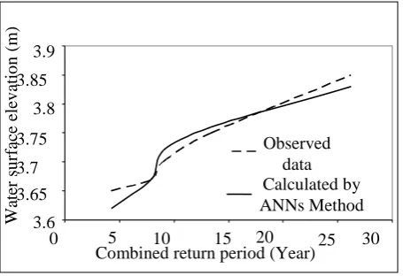
Observed data are water surface elevations in Salmanieh Station. The observed data and calculated water surface elevations by ANN method are shown in Fig. 8.
Fig. 8 Observed data and calculated water surface elevations by ANN method
4 4.1 4.2 4.3 4.4 4.5 4.6
165 167 169 171 173 175 177 179
Distance from Ahvaz (Km)
W
at
er
s
u
rf
ac
e
el
ev
at
io
n
(
m
)
Conventional method Structural curves method Structural regression relations method Neural network method
Fig. 9 Comparison between results of four methods for combined return period 100 years
3.5 Comparison between Results of Four
Methods
Comparison between results of four methods is shown in Fig. 9 for combined return period 100 years. Fig. 9 shows that difference between calculated water surface elevations by conventional method and other methods are approximately 10 Cm. This amount seems insignificant but this small amount can reduce volume and cost of construction of flood wall and dikes considerably. If width of flood wall is one meter, volume of flood wall will reduce 100 cubic meters at per kilometer. By attention to long length of river, selection of suitable method for calculation of water surface elevation is essential for economic savings.
4. Conclusion
Results of conventional method are very conservative. This method considers two extremely states. Results of other three methods are similar. Neural network method is a simple and accurate method. Results of neural network method have good adjustment with observed data. This adjustment can be seen in a great range of combined return periods. If neural network is trained well, it will be the best method for determination of water surface elevation in tidal limit of tidal rivers. A suitable ANN can be found for each tidal river. This ANN can show maximum water surface elevation in each section of tidal limit for different boundary conditions and different combined return periods while numerical models do not show correct water surface elevation in this part of tidal river.
References
[1] Godin, G. Modification of river tides by the discharge. Journal of Waterway, Port, Coastal, and Ocean Engineering, ASCE, Volume 111(2), (1985), pp. 257-274.
[2] Vongvisessomjai, S., and Rojanakamthorn, S. Interaction of tide and river flow. Journal of Waterway, Port, Coastal, and Ocean Engineering, ASCE, Volume 115(1), (1989), pp. 86-104. [3] Sobey, R.J. Evaluation of numerical models of
flood and tide propagation in channels. Journal of Hydraulic Engineering, ASCE, Volume 127(10), (2001), pp. 805-824.
[4] Sanders, B.F., Green, C.L., Chu, A.K., and Grant, S.B. Case study: modeling tidal transport of urban runoff in channels using the finite-volume method. Journal of Hydraulic Engineering, ASCE, Volume 127(10), (2001), pp. 795-804.
[5] Samuels, P.G., and Burt, N. A new joint probability appraisal of flood risk. Proceedings of the Institution of Civil Engineers- Water and Maritime Engineering, Volume 154(2), (2002), pp. 109-115.
[6] Acreman, M.C. Assessing the joint probability of fluvial and tidal floods in the river Roding. Water 3.6
3.65 3.7 3.75
3.8 3.85
3.9
0 5 10 15 20 25 30
Combined return period (Year)
W
ater
s
u
rf
ac
e
elev
atio
n
(
m
)
and Environment Journal, Volume 8(5), (1994), pp. 490-496.
[7] Mantz, P.A., and Wakeling, H.L. Forecasting flood levels for joint events of rainfall and tidal surge flooding using extreme value statistics. Proceedings of the Institution of Civil Engineers, Volume 67(1), (1979), pp. 31-50.
[8] Liang, S.X., Li, M.C., and Sun, Z.C. Prediction models for tidal level including strong meteorologic effects using a neural network. Ocean Engineering, Volume 35(7), (2008), pp. 666-675.
[9] Pashova, L., and Popova, S. Daily sea level forecast at tide gauge Burgas, Bulgaria using artificial neural networks. Journal of Sea Research, Volume 66(2), (2011), pp. 154-161. [10] Remya, P.G., Kumar, R., and Basu, S. Forecasting
tidal currents from tidal levels using genetic algorithm. Ocean Engineering, Volume 40, (2012), pp. 62-68.
[11] Adib, A., and Nasiriyani, M.Evaluation of fluvial flow effects on tidal characteristics of tidal rivers by artificial neural networks and genetic algorithm. International Journal of Water, Volume 10(1), (2016), pp. 13-27.
[12] Adib, A., and Jahanbakhshan, H. Stochastic approach to determination of suspended sediment concentration in tidal rivers by artificial neural network and genetic algorithm. Canadian Journal of Civil Engineering, Volume 40(4), (2013), pp. 299-312.
[13] Adib, A., and Javdan, F. Interactive approach for determination of salinity concentration in tidal rivers (Case study: The Karun River in Iran). Ain Shams Engineering Journal, Volume 6(3), (2015), pp. 785-793.
[14] Liu, W.C., Chan, W.T., and Young, C.C. Modeling fecal coliform contamination in a tidal Danshuei River estuarine system. Science of The Total Environment, Volume 502, (2015), pp. 632-640.
[15] Wang, Y., Liu, Z., Gao, H., Ju, L., and Guo, X. Response of salinity distribution around the Yellow River mouth to abrupt changes in river discharge. Continental Shelf Research, Volume 31(6), (2011), pp. 685-694.
[16] Shi, J.Z., and Zhang, H.L. Passage of the partially-mixed Changjiang River estuary, China. Journal of
Hydro-Environment Research, Volume 5(1),
(2011), pp. 49-62.