Preprocessing differential methylation hybridization microarray data

(1)

M E T H O D O L O G Y

Open Access

Preprocessing differential methylation

hybridization microarray data

Shuying Sun

1,2*

, Yi-Wen Huang

3

, Pearlly S Yan

3

, Tim HM Huang

3

and Shili Lin

4

* Correspondence: [email protected]

1_{Case Comprehensive Cancer}

Center, Case Western Reserve University, Cleveland, Ohio, 44106, USA

Full list of author information is available at the end of the article

Abstract

Background:DNA methylation plays a very important role in the silencing of tumor suppressor genes in various tumor types. In order to gain a genome-wide

understanding of how changes in methylation affect tumor growth, the differential methylation hybridization (DMH) protocol has been developed and large amounts of DMH microarray data have been generated. However, it is still unclear how to preprocess this type of microarray data and how different background correction and normalization methods used for two-color gene expression arrays perform for the methylation microarray data. In this paper, we demonstrate our discovery of a set of internal control probes that have log ratios (M) theoretically equal to zero

according to this DMH protocol. With the aid of this set of control probes, we propose two LOESS (or LOWESS, locally weighted scatter-plot smoothing) normalization methods that are novel and unique for DMH microarray data. Combining with other normalization methods (global LOESS and no normalization), we compare four normalization methods. In addition, we compare five different background correction methods.

Results:We study 20 different preprocessing methods, which are the combination of five background correction methods and four normalization methods. In order to compare these 20 methods, we evaluate their performance of identifying known methylated and un-methylated housekeeping genes based on two statistics. Comparison details are illustrated using breast cancer cell line and ovarian cancer patient methylation microarray data. Our comparison results show that different background correction methods perform similarly; however, four normalization methods perform very differently. In particular, all three different LOESS normalization methods perform better than the one without any normalization.

Conclusions:It is necessary to do within-array normalization, and the two LOESS normalization methods based on specific DMH internal control probes produce more stable and relatively better results than the global LOESS normalization method.

Background

Microarray technology has been used extensively in genetic and epigenetic studies over the last ten years. Several microarray platforms are available including the single-channel Affymetrix oligonucleotide arrays, the two-color (or two-channel) cDNA arrays, and Agilent two color arrays. In the two-color use, which is the focus of this paper, two sam-ples (or target genes) are labeled using two different fluorophores (usually a red fluores-cent dye, Cy5, and a green fluoresfluores-cent dye, Cy3) and hybridized simultaneously onto each probe (or spot) of the array (or chip). Then the arrays are laser-scanned and images

(2)

are processed to obtain the data for analysis [1]. In general, the log ratio Cy5 over Cy3 at each probe is used as a measurement. With this microarray technology, studying thou-sands of genes simultaneously becomes possible. For example, gene expression, copy number variation, and methylation patterns have been widely studied using microarray technologies. However, due to some experimental artifacts, random noise and systematic variation do exist in such high throughput microarray experiments. Therefore, prepro-cessing, such as background correction and normalization, is important to eliminate technical bias in order to identify real biological variations.

Preprocessing gene expression microarray data obtained from two-color cDNA microarray and single-color Affymetrix array have been extensively studied [2-4]. However, two-color methylation microarrays, especially the DNA methylation micro-arrays generated based on the DMH protocol [5-7] with the Agilent technology [8], have not been well studied. DNA methylation arrays are very different from gene expression arrays. The differences mainly lie in the following two aspects. First, dif-ferent materials are hybridized onto the array. For the gene expression array, it is the mRNA that is reverse transcribed to cDNA. While for the DNA methylation microarray, it is the DNA fragments selected based on the methylation-sensitive restriction enzymes (MSRE) [5,7,9-11] or methyl-cytosine-specific antibody [12-15]. Second, they measure different biological phenomena, one measures gene expression, or the mRNA levels, and another measures methylation signals. It has been recog-nized that preprocessing methods for microarrays are platform specific and challen-ging to automate [2,16]. It is still unknown whether gene expression array preprocessing methods can be applied to the Agilent two-color methylation microar-ray. If applied, it is not clear how different background correction and normalization methods would perform.

After the image analysis, foreground and background intensities are estimated for each probe (or spot), and these intensities are usually denoted as Rf, Gf, Rb, and Gb

respectively for the two channels (i.e., the red and green channels). The foreground estimates (Rfand Gf) are the overall measurement of the intensity at each probe (spot)

in each channel. The background measurements (Rb, Gb) are usually an estimate of the

ambient signal around the round circle of each spot. This may be due to unequal dis-tribution of hybridization solution, spatial bias [17], non-specific binding of labeled samples to the array surface, or non-hybridized DNA not washed away [18]. Removing these ambient signals around each probe and adjusting the foreground signals accord-ingly is called background correction.

(3)

correction (i.e., subtraction) performs far worse than other alternatives in that it produces a larger number of false discoveries. Ritchie et al. [18] also shows that variance stabiliza-tion methods perform best, especially the‘normexp+offset’method, which gives the lowest false discovery rate. Whether these conclusions are valid in the methylation data generated by the Agilent technology is still unknown. In addition, Ritchie et al. [18] only compare background correction methods and do not demonstrate how normalization methods will affect and interact with different background correction methods.

In order to obtain accurate measurements from microarray technology, we must consider the random and systematic variation due to some experimental artifacts. Nor-malization of microarray data is the process of removing or adjusting these systematic biases that usually include intensity dependent bias, dye bias and spatial effects [2,4]. A commonly used normalization method is the intensity dependent LOESS normaliza-tion that fits a locally weighted polynomial regression to the average of the red and green intensities, that is, the LOESS curve [2,4]. This LOESS normalization generally involves two steps [23]: (1) select probes (or genes) used to do normalization, and (2) apply a LOESS or weighted LOESS to the data. The probes or genes that are normally selected are all probes (genes), the housekeeping genes, the spike-in control probes, and microarray sample pool control (MSP). Housekeeping genes have originally been used for normalization because they are believed to have stable function and stable gene expression values. However, it has been shown that they have large variability between different samples and treatments [24,25]. Spike-in controls may be more trustworthy, but not all microarray experiments have included spike-in controls. Microarray sample pool controls [2] are designed for gene expression data normaliza-tion, and their performance is still unknown for methylation data. To the best of our knowledge, no probes or genes are selected specifically for normalizing DMH microar-ray data.

In this paper, we demonstrate the identification of a set of probes that are specially selected as internal control probes for the DMH protocol. Utilizing these DMH internal control probes, we propose two LOESS normalization methods that are novel and unique for the DMH methylation microarray data. Combining these two control probe LOESS methods with other two standard normalization methods (global LOESS normalization and no normalization), we compare four normalization methods. In addition, we also compare five different background correction methods. Combining all these different background correction and normalization methods results in 20 different preprocessing methods for the DNA methylation microarrays. In order to see which preprocessing method can best identify known methylated and housekeeping genes, all 20 methods are compared using microarray data generated from breast cancer cell lines and ovarian cancer patients.

Results

DMH microarray protocol and data sets

(4)

genome. This assay includes the following three steps. More details of the description of the DMH protocols can be found in the literature [5-7,26].

1) Sonicating DNA sequences into 400-500 bp fragments, and then ligating these fragments using linkers.

2) Digesting ligated DNA fragments using two MSREs, HpaII and HinpI, which have the recognition cutting sites CCGG and CGCG respectively. If a DNA frag-ment contains at least one recognition cutting site that is not methylated, it will be restricted (i.e., cut), and will not be hybridized onto the microarray. Therefore, it does not contribute to the final methylation signals.

3) Using the polymerase chain reaction (PCR) to amplify the unrestricted DNA fragments and then hybridizing them onto microarrays.

The above three steps are done for both test (cancer patients or cell lines) and con-trol (common normal references) samples. Then both samples are hybridized to the array coupled with red or green fluorescent dyes. Here we use the Agilent 244K arrays hybridized with the test samples (e.g., cancer cell lines) labeled with Cy5 (red dye, or R) and a common normal reference labeled with Cy3 (green dye, or G). Two color arrays produce both foreground, i.e., Rf and Gf, and background, i.e., Rband Gb,

inten-sities. After some proper background correction and normalization based on Rf, Gf, Rb

and Gb, we obtain the true signals R and G. We use the base two log ratio of red over

green intensity, log2(R/G), as the observed methylation signal at each probe. This is

called the M value, that is, log2(R) - log2(G). The average is (log2(R) + log2(G))/2 and

is called the A value. The MA plot (with A values in the x-axis and M values in the y-axis) is often used to examine dye bias before doing any normalization.

In this paper, we study 20 different preprocessing methods that are the combination of five-background correction and four normalization methods. These comparisons are done using two microarray data sets from 40 breast cancer cell lines and 26 ovarian can-cer patients. For each array in these two data sets, we preprocess it with different back-ground correction and normalization methods and then examine which preprocessing method is better at identifying known methylated and non-methylated genes. For the breast cancer cell line data, 30 known methylated genes [27-30] are used. For the ovarian cancer data, 32 known methylated genes are selected [31]. For the non-methylated genes, we use 47 known housekeeping genes selected from publicly available data [32].

Review of background correction methods

1) None: no background correction and simply let R = Rf and G = Gf.

2) Subtract: this is the traditional background correction method with the local background estimate subtracted from the foreground estimate. That is, R = Rf- Rb

and G = Gf- Gb.

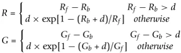
3) Edwards: in order to avoid the situation of local background estimates less than foreground estimates, Edwards [17] proposes to subtract background (Rband Gb)

from foreground (Rfand Gf) when their difference is larger than a certain threshold

(5)

R=

Rf −Rb Rf −Rb>d

d×exp[1−(Rb+d)/Rf] otherwise

G=

Gf−Gb Gf −Gb>d

d×exp[1−(Gb+d)/Gf] otherwise

4) Normexp: this method applies a normal-exponential (i.e., normexp) convolution model to the local background and the true signal at the red and green channels separately [18,22]. For example, at the red channel, let S be the unknown true sig-nal, let B be the background noise that is not included in Rb, and let X = Rf-Rbbe

the background-corrected observed intensity. According to the normexp model, S ~ exp(a) (i.e., an exponential distribution with meana), B ~N(μ,s2) (i.e., a normal distribution with meanμand variance s2), and S and B are independent and addi-tive. Therefore, we have X = S + B. We can derive the intensity function for S and X, and then the conditional density of S|X. The estimate of the unknown true sig-nal S is the conditiosig-nal expectation E(S|X = x). The three key parameters,a,μand

s2

, can be estimated using a saddle-point approximation or the maximum likeli-hood method [18,22]. The true signals in red and green channels, which are usually denoted as R and G, can be obtained and their log ratio, log2(R/G), will be used as the methylation signal at each probe.

5) Normexp+offset: this is the same as the Normexp method except that a small positive offset is added to both channels to reduce the variance of low intensity log ratio values. That is, the new log ratio value is equal to log2[(R+k)/(G+k)]. As used in [18], we let k = 50.

Novel and existing normalization methods

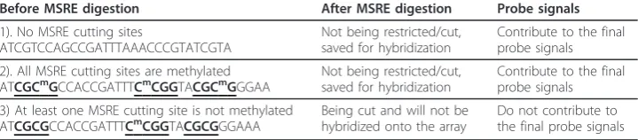
The basic rationale of normalization is to remove or adjust for artifacts caused by microarray technology rather than biological differences of the samples between printed probes. In order to do so, it is helpful to normalize the data with some known information, for example, some control probes that are known to be non-differentially methylated. In this section, we first identify the probes that are known to be not differ-entially methylated based on the DMH protocol, that is, probes with M = 0. DNA frag-ments are restricted by two MSREs, HinpI and HapII, which have the recognition cutting sites CGCG and CCGG respectively. If a DNA fragment contains at least one cutting site that is not methylated, it will be restricted (i.e., cut), and will not be hybri-dized onto the microarray. If a DNA fragment does not have any cutting sites, it will not be digested by any MSREs and can be hybridized onto the array. If all the cutting sites of a DNA fragment are methylated, this fragment will be saved for hybridization onto the array. These three typical types of DNA fragments with examples are given in Table 1.

(6)

probe, we check the regions that are L = 900 bases around the center of each probe. That is, there are L/2 bases on each side of the center of the probe. Then we check how many restriction cutting sites are around this probe within these L bases. If there are no cutting sites (i.e., the sequences CGCG and CCGG), we claim that this probe is a non-differential methylated internal control probe with M = 0. These internal control probes are important because we can make full use of them to do normalizations. Because the length of DNA fragments is about 400-500 bp, we use L = 900 bases assuming that DNA fragments can be hybridized onto the methylated probes and regions evenly. 199 probes, which have no recognition cutting sites around 900 bp, are identified.

Similar to the LOESS normalization and composite LOESS normalization using con-trol probes in the context of the gene expression microarray preprocessing, we intro-duce the control and composite LOESS normalization for DMH methylation microarray data. Combining with the standard LOESS normalization and the method without any normalization, there are four normalization methods. Details about these four normalization methods are described as below:

1) None: no normalization is done, and Mnew= Mobserved.

2) Global LOESS normalization: all the biological probes are used, and Mnew =

Mobserved-fLOESS(A).

3) Control LOESS normalization: We fit a LOESS curve only using the 199 control probes, and for each M value which corresponds to an A value, we have Mnew =

M- fcontrol(A).

4) Composite LOESS normalization: This is to let the normalization curve to be a weighted average of the global LOESS curve and the control probe LOESS curve. That is, at each specific average intensity level A, the new normalized estimate is g (A) = a* fcontrol(A) + (1-a) fall(A), and Mnew= Mobserved- g(A), where falland fcontrol

are the global and control LOESS curve, and ‘a’ is defined as the proportion of genes less than a given intensity A value [2].

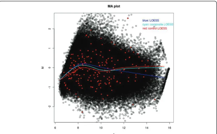
In Figure 1, we show an example of the MA plot of an array that is fitted with three different LOESS curves: global LOESS (blue line), composite LOESS (cyan line), and control LOESS (red line). This figure shows that there are some differences among these three LOESS curves, so the normalization based on these three LOESS curves could be very different. In this Figure, the red dots are the 199 internal control probes with M = 0 as their theoretical log ratio values according to our DMH protocol. As we

Table 1 Examples of three types of DNA fragments

Before MSRE digestion After MSRE digestion Probe signals

1). No MSRE cutting sites

ATCGTCCAGCCGATTTAAACCCGTATCGTA

Not being restricted/cut, saved for hybridization

Contribute to the final probe signals

2). All MSRE cutting sites are methylated

ATCGCm_GCCACCGATTTCm_CGGTACGCm_GGGAA Not being restricted/cut,_{saved for hybridization} Contribute to the final_{probe signals}

3) At least one MSRE cutting site is not methylated

ATCGCGCCACCGATTTCm_{CGGTACGCGGGAAA} Being cut and will not be_{hybridized onto the array} Do not contribute to_{the final probe signals}

(7)

see that some probes have some unexpected large and small log ratios, this could be due to some experimental artefacts. Therefore, we should preprocess the raw microar-ray data first.

Comparison methods

All 20 different preprocessing methods as described are implemented using the LIMMA package [4] of Bioconductor [33]. In order to compare the different back-ground and normalization methods, we use the quantile regression method [34], which identifies commonly hypermethylated genes in DMH microarray data. The basic idea is that, for each CpG island we apply the quantile regression model [35] to the normal-ized M values obtained from 20 different preprocessing methods. Then we use some known methylated genes and 47 un-methylated housekeeping genes as positive and negative controls to see which preprocessing method is better at identifying these two different groups of genes (methylated and non-methylated). At each CpG island, we fit a 75% quantile regression with the array (or cell line, patients) and probes as

covari-ates, that is, Map= arraya+probep+ errorap,

P p=1

probep= 0, all error terms are assumed

to be independent and distribution free. Both“array”and “probe” are fixed effects. For each array (cell line or patient), we obtain a p-value from the quantile regression out-put to indicate whether there is some hypermethylation signal at 75% quantile for each array. The methylation score given to each CpG island is the count of the number of cell lines with p-value less than a certain threshold p0, where we let p0 = 0.05, 0.04,

0.03, 0.02 and 0.01. At each p-value threshold p0, we have an integer methylation score

n for each CpG island. The range of n is from 0 to N, where N is 40 and 26 for breast cancer cell line data and ovarian cancer data respectively. There are in total of Nmand

(8)

NHKmethylation scores for known methylated genes/CpG islands (Nm= 30 for breast

cancer data, Nm = 32 for ovarian cancer) and housekeeping genes (NHK = 47)

respectively.

In order to see if known methylated genes and housekeeping genes are identified correctly, we use two different statistical measurements for known methylated genes and housekeeping genes. One is the statistics of mean difference of methylation scores

of two groups of genes divided by their variance. That is, ¯

xm− ¯xHK

s2

m/Nm+s2_HK/NHK

, where

¯

xHK, x¯HK, s2m and s2HKare the mean and variance of methylation scores for known

methylated genes and housekeeping genes respectively, we call this measurement “T. stat”. Another measurement is the area under the Receiver Operating Characteristic (ROC) curve, and we call it “AUC”. For each preprocessing method, the AUC is calcu-lated according to the false positive and true positive rates defined in the following way. At each methylation level C0 that ranges from 0 to N, the false positive rate is the

ratio of the number of un-methylated housekeeping genes/CpG islands with methyla-tion scores greater than or equal to C0 and the total number of housekeeping genes

(NHK), and the true positive rate is the ratio of the number of known methylated

genes/CpG islands with methylation scores greater than or equal to C0 and the total

number of known methylated genes (Nm). For both T.stat and AUC, the larger a

statis-tical measurement is, the better a processing method is.

Comparison results

(9)

the combination of background subtraction and control LOESS work slightly better than the others.

In order to further compare the performances of different normalization and back-ground correction methods, at each p-value cutoff point we calculate the average of each statistical measurement for each normalization method (across five different back-ground correction methods) and for each backback-ground correction method (across four different normalization methods). The average scores are plotted in Figure 2 (for breast cancer data) and Figure 3 (for Ovarian cancer data). In each of these two figures, two plots in the top panel are used to compare four different normalization methods using measurements T.stat and AUC. Two plots in the bottom panel are used for the com-parisons of five different background correction methods using measurements T.stat and AUC. Both Figures 2 and 3 show that there are more differences among normali-zation methods than among background correction methods. If we ignore the LOESS normalization method, that is, the blue line in plots A and C of Figures 2 and 3, we can see that the performance of the other three normalization methods can be ranked in the following order in both breast cancer and ovarian cancer data: control LOESS (red curve) is better than composite LOESS which is better than “none” (i.e., without any normalization). The global LOESS normalization method is less efficient than the composite LOESS method in breast cancer data, but it is better than the composite LOESS method in ovarian cancer data, in which control LOESS and global LOESS

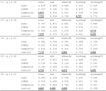
Table 2 Breast cancer T.stat measurement table

(1): p < 0.05 none sub edwards normexp normexp50

none 4.879 4.896 4.880 6.010 6.065

LOESS 6.037 5.786 5.783 5.875 5.923

composite 6.872 6.410 6.423 6.508 6.598

control 7.753 6.516 6.738 6.797 6.771

none 4.747 4.871 4.855 6.012 5.889

LOESS 5.725 5.928 5.951 5.579 5.711

composite 6.565 6.230 6.279 6.426 6.716

control 7.570 6.371 6.622 6.691 6.959

none 4.665 4.766 4.761 5.484 5.758

LOESS 5.621 5.534 5.544 5.367 5.377

composite 6.602 6.330 6.305 6.065 6.629

control 7.110 6.573 6.865 6.730 6.966

none 4.237 4.457 4.444 5.488 5.493

LOESS 5.134 5.184 5.109 4.980 5.063

composite 6.385 6.049 6.026 5.953 6.335

control 6.734 6.471 6.673 6.504 6.695

none 4.094 4.318 4.304 5.207 5.260

LOESS 5.063 4.966 4.938 4.651 4.796

composite 6.252 6.040 6.080 5.566 5.927

control 6.662 6.484 6.694 6.435 6.398

(10)

have similar performance. Plots B and D in both Figures 2 and 3 show that the ence between different background correction methods is not very much, their differ-ence is much smaller than the differdiffer-ences among four normalization methods.

Conclusions and Discussion

In this paper, we compare four normalization and five background correction methods. There are more differences among normalization methods than background correction methods. Among four normalization methods, the result of no normalization performs the worst in that both statistical measurement scores are the smallest in both data sets. Therefore, it is necessary to do normalization. The control LOESS and composite LOESS normalization methods provide relatively stable results in both data sets when the p value threshold changes. However, the LOESS normalization results are more variable across different p-value cutoff points. On the other hand, the differences among background correction methods are relatively small. Our comparison results show that even though some background correction methods are slightly better than others, the differences are much smaller than the differences among normalization methods. With appropriate normalization, the need for background-corrected DMH methylation data might be obviated. This conclusion is consistent with the findings of [8], which are about the gene expression microarray data. That is, differentially expressed genes are most reliably detected when background is not subtracted. It is

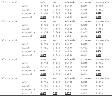
Table 3 Breast cancer AUC measurement table

none 0.779 0.782 0.781 0.841 0.842

LOESS 0.852 0.842 0.841 0.868 0.861

composite 0.864 0.849 0.849 0.868 0.872

control 0.896 0.854 0.859 0.869 0.875

none 0.773 0.775 0.774 0.848 0.830

LOESS 0.846 0.855 0.855 0.851 0.854

composite 0.856 0.844 0.846 0.867 0.882

control 0.896 0.849 0.854 0.866 0.883

none 0.763 0.771 0.771 0.815 0.830

LOESS 0.851 0.836 0.836 0.841 0.835

composite 0.862 0.852 0.850 0.860 0.884

control 0.877 0.861 0.868 0.869 0.879

none 0.738 0.751 0.751 0.818 0.826

LOESS 0.826 0.823 0.816 0.818 0.832

composite 0.866 0.837 0.834 0.854 0.873

control 0.866 0.853 0.854 0.864 0.871

none 0.736 0.730 0.730 0.810 0.796

LOESS 0.844 0.820 0.817 0.814 0.837

composite 0.868 0.851 0.852 0.826 0.857

control 0.871 0.871 0.872 0.861 0.863

(11)

also consistent with the conclusion of [36], which claims that background correction is generally needed to remove bias, but appropriate normalization obviates the need for mock experiments.

The housekeeping genes used as non-methylated genes are selected from publicly avail-able data [32] using the following criteria. First, there is one and only one CpG island asso-ciated with this gene. We use this criterion because there could be several CpG islands associated with one housekeeping gene, in this case we cannot determine the methylation signal of such housekeeping gene. Second, there are at least three probes and at least one probe is in the promoter region according to the annotation provided by Agilent. We use this standard because methylation signals at CpG island with small number of probes are not reliable according to our previous work [26]. Third, the CpG island associated with a housekeeping gene will have a methylation score less than or equal to N/2 (that is, half of the number of arrays) in all 20 preprocessing methods and in the data of both breast and ovarian cancer. We choose housekeeping genes in this way to avoid any bias due to pre-processing methods and cancer types. Housekeeping genes could have large variability between different samples and treatments [24,25], especially in cancer tumor or cell lines. For example, some housekeeping genes may have abnormally high or low expression and/ or methylation level in breast cancer but not in ovarian cancer.

In Table 2 of the ovarian cancer methylation review paper [31], 49 genes are sum-marized as hypermethylated genes. In our comparisons, we only use 32 of them. The

Table 4 Ovarian cancer T.stat measurement table

none 4.451 4.618 4.618 4.033 4.406

LOESS 5.834 5.968 6.055 5.629 5.605

composite 5.138 5.159 5.159 5.112 5.311

control 5.834 6.166 6.083 5.703 5.623

none 4.489 4.629 4.629 4.249 4.348

LOESS 5.814 5.734 5.828 5.501 5.538

composite 5.157 5.385 5.261 5.177 5.059

control 5.738 6.193 6.106 5.627 5.440

none 4.645 4.548 4.548 4.589 4.452

LOESS 5.681 5.890 5.890 5.618 5.532

composite 5.316 5.491 5.491 4.977 4.885

control 5.657 5.803 5.781 5.554 5.520

none 4.761 4.614 4.652 4.389 4.560

LOESS 5.758 5.862 5.888 5.503 5.128

composite 5.315 5.255 5.242 4.848 4.953

control 5.621 5.873 5.912 5.602 5.627

none 4.834 4.662 4.699 4.196 4.298

LOESS 5.330 5.416 5.416 5.033 4.903

composite 5.304 5.114 5.126 4.769 4.559

control 5.736 5.924 5.893 5.381 5.371

(12)

other 17 genes are excluded for one or more of the following reasons: (1) there is no corresponding CpG island in our methylation microarray data, (2) the corresponding CpG island has less than 3 probes, (3) the corresponding CpG island does not cover the promoter or first exon region of this gene according to the annotation provided by Agilent, or (4) there are several CpG islands corresponding to this gene, and it is diffi-cult to select one.

The effectiveness of a normalization method depends on whether or not its assump-tion is valid. The LOESS normalizaassump-tion assumes that each array has a larger number of probes (or genes) that are not differentially methylated (expressed), or there is an approximately equal number of positive and negative log ratios. It also requires that a certain number of probes with these characteristics should cover a full range of intensi-ties [37]. However, these assumptions could fail in the breast cancer cell line methylation data since cell lines usually have more methylation than patients. This might be one main reason that the control LOESS normalization and composite LOESS normalization are better (i.e., provide more stable results) than the global LOESS normalization for some p-value cutoff values in the breast cancer cell line data, but not in the ovarian can-cer data. In addition, copy number variations may occur in cancan-cer patient tumor and cell lines. This may be one of the reasons that those internal control probes may have unexpected large or small log ratios. However, it is unlikely that the log-ratios of all

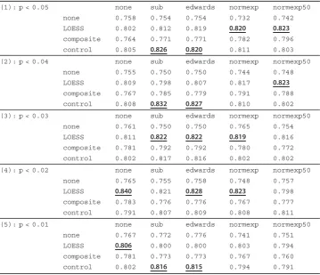
Table 5 Ovarian cancer AUC measurement table

none 0.758 0.754 0.754 0.732 0.742

LOESS 0.802 0.812 0.819 0.820 0.823

composite 0.764 0.771 0.771 0.782 0.796

control 0.805 0.826 0.820 0.811 0.803

none 0.755 0.750 0.750 0.744 0.748

LOESS 0.809 0.798 0.807 0.817 0.823

composite 0.767 0.785 0.779 0.791 0.788

control 0.808 0.832 0.827 0.810 0.802

none 0.761 0.750 0.750 0.765 0.754

LOESS 0.811 0.822 0.822 0.819 0.816

composite 0.781 0.792 0.792 0.780 0.772

control 0.802 0.817 0.816 0.802 0.802

none 0.765 0.755 0.758 0.748 0.757

LOESS 0.840 0.821 0.828 0.823 0.798

composite 0.783 0.776 0.776 0.767 0.777

control 0.791 0.807 0.809 0.808 0.811

none 0.767 0.772 0.776 0.741 0.751

LOESS 0.806 0.800 0.800 0.803 0.794

composite 0.781 0.773 0.773 0.767 0.760

control 0.802 0.816 0.815 0.794 0.791

(13)

A: Normalization (T.stat)

$# #" ##"#" ""$ #!! "#!

B: Background Correction (T.stat)

$# #"

##"#"

"$$

%!

!& ! !& $!

C: Normalization (AUC)

$# #" ""$ #!! "#!

D: Background Correction (AUC)

$# #" "$$ %! !& ! !& $!

Figure 2Breast cancer mean differences of different normalization and background correction methods. The two plots in the top panel are the results of comparing four normalization methods using two statistical measurements. The two plots in the bottom panel are the results of comparing five background correction methods using two statistical measurements.

A: Normalization (T.stat)

$# #" ##"#" ""$ #!! "#!

B: Background Correction (T.stat)

$# #" ##"#" "$$ %! !& ! !& $!

C: Normalization (AUC)

$# #" ""$ #!! "#!

D: Background Correction (AUC)

$# #" "$$ %! !& ! !& $!

(14)

those 199 internal probes will be affected, so copy number variations may not affect the validity of our results.

In this paper, we did not compare with the Agilent Feature Extraction Software [38] because it has been shown that it does not outperform the LOESS normalization [8]. Although the internal control probes we identified are mainly used for preprocessing DMH data in this paper, the ideas of our methods can be useful for preprocessing data generated from other methylation microarray and sequencing protocols [10,11,39,40] that use methylation sensitive or insensitive enzymes to digest DNA fragments.

Acknowledgements

This work was supported by the National Science Foundation [0112050] while SS was a postdoctoral researcher in the Mathematical Biosciences Institute, The Ohio State University. The authors thank Drs. Terry Speed, Greg Singers and Dustin Potter for valuable suggestions and discussions. In particular, we appreciate that Dr. Potter shared the methylation-sensitive restriction enzyme cutting sites data (from his previous DMH publications) with us.

Author details

1

Case Comprehensive Cancer Center, Case Western Reserve University, Cleveland, Ohio, 44106, USA.2Department of Epidemiology and Biostatistics, Case Western Reserve University, Cleveland, Ohio, 44106, USA.3_{Human Cancer}

Genetics Program, The Ohio State University, Columbus, Ohio, 43210, USA.4Department of Statistics, The Ohio State University, Columbus, Ohio, 43210, USA.

Authors’contributions

SS developed and implemented the models, performed all statistical analyses, drafted and revised the manuscript. PSY and YWH were involved in the data collection and helped in preparation of the manuscript. THMH oversaw the project and revised the manuscript. SL provided suggestions on the project and revised the manuscript. All authors have read and approved the final document.

Competing interests

The authors declare that they have no competing interests.

Received: 17 November 2010 Accepted: 16 May 2011 Published: 16 May 2011

References

1. Duggan DJ, Bittner M, Chen Y, Meltzer P, Trent JM:Expression profiling using cDNA microarrays.Nature Genetics1999,

21(1 Suppl):10-14.

2. Yang YH, Dudoit S, Luu P, Lin DM, Peng V, Ngai J, Speed TP:Normalization for cDNA microarray data: a robust composite method addressing single and multiple slide systematic variation.Nucleic Acids Res2002,30(4):e15. 3. Irizarry RA, Hobbs B, Collin F, Beazer-Barclay YD, Antonellis KJ, Scherf U, Speed TP:Exploration, normalization, and

summaries of high density oligonucleotide array probe level data.Biostatistics2003,4(2):249-264. 4. Smyth GK, Speed T:Normalization of cDNA microarray data.Methods2003,31(4):265-273.

5. Huang TH, Perry MR, Laux DE:Methylation profiling of CpG islands in human breast cancer cells.Hum Mol Genet

1999,8(3):459-470.

6. Yan PS, Chen CM, Shi H, Rahmatpanah F, Wei SH, Huang TH:Applications of CpG island microarrays for high-throughput analysis of DNA methylation.J Nutr2002,132(8 Suppl):2430S-2434S.

7. Yan PS, Potter D, Deatherage DE, Huang TH, Lin S:Differential methylation hybridization: profiling DNA methylation with a high-density CpG island microarray.Methods Mol Biol2009,507:89-106.

8. Zahurak M, Parmigiani G, Yu W, Scharpf RB, Berman D, Schaeffer E, Shabbeer S, Cope L:Pre-processing Agilent microarray data.BMC Bioinformatics2007,8:142.

9. Estecio MR, Yan PS, Ibrahim AE, Tellez CS, Shen L, Huang TH, Issa JP:High-throughput methylation profiling by MCA coupled to CpG island microarray.Genome Res2007,17(10):1529-1536.

10. Irizarry RA, Ladd-Acosta C, Carvalho B, Wu H, Brandenburg SA, Jeddeloh JA, Wen B, Feinberg AP:Comprehensive high-throughput arrays for relative methylation (CHARM).Genome Res2008,18(5):780-790.

11. Khulan B, Thompson RF, Ye K, Fazzari MJ, Suzuki M, Stasiek E, Figueroa ME, Glass JL, Chen Q, Montagna C, Hatchwell E, Selzer RR, Richmond TA, Green RD, Melnick A, Greally JM:Comparative isoschizomer profiling of cytosine

methylation: the HELP assay.Genome Res2006,16(8):1046-1055.

12. Keshet I, Schlesinger Y, Farkash S, Rand E, Hecht M, Segal E, Pikarski E, Young RA, Niveleau A, Cedar H, Simon I:

Evidence for an instructive mechanism of de novo methylation in cancer cells.Nat Genet2006,38(2):149-153. 13. Weber M, Davies JJ, Wittig D, Oakeley EJ, Haase M, Lam WL, Schubeler D:Chromosome-wide and promoter-specific

analyses identify sites of differential DNA methylation in normal and transformed human cells.Nat Genet2005,

37(8):853-862.

14. Weber M, Hellmann I, Stadler MB, Ramos L, Paabo S, Rebhan M, Schubeler D:Distribution, silencing potential and evolutionary impact of promoter DNA methylation in the human genome.Nat Genet2007,39(4):457-466. 15. Zhang X, Yazaki J, Sundaresan A, Cokus S, Chan SW, Chen H, Henderson IR, Shinn P, Pellegrini M, Jacobsen SE, Ecker JR:

Genome-wide high-resolution mapping and functional analysis of DNA methylation in arabidopsis.Cell2006,

(15)

16. Tseng GC, Oh MK, Rohlin L, Liao JC, Wong WH:Issues in cDNA microarray analysis: quality filtering, channel normalization, models of variations and assessment of gene effects.Nucleic Acids Res2001,29(12):2549-2557. 17. Edwards D:Non-linear normalization and background correction in one-channel cDNA microarray studies.

Bioinformatics2003,19(7):825-833.

18. Ritchie ME, Silver J, Oshlack A, Holmes M, Diyagama D, Holloway A, Smyth GK:A comparison of background correction methods for two-colour microarrays.Bioinformatics2007,23(20):2700-2707.

19. Tran PH, Peiffer DA, Shin Y, Meek LM, Brody JP, Cho KW:Microarray optimizations: increasing spot accuracy and automated identification of true microarray signals.Nucleic Acids Res2002,30(12):e54.

20. Yin W, Chen T, Zhou SX, Chakraborty A:Background correction for cDNA microarray images using the TV+L1 model.

Bioinformatics2005,21(10):2410-2416.

21. Kooperberg C, Fazzio TG, Delrow JJ, Tsukiyama T:Improved background correction for spotted DNA microarrays.

J Comput Biol2002,9(1):55-66.

22. Silver JD, Ritchie ME, Smyth GK:Microarray background correction: maximum likelihood estimation for the normal-exponential convolution.Biostatistics2009,10(2):352-363.

23. Chua SW, Vijayakumar P, Nissom PM, Yam CY, Wong VV, Yang H:A novel normalization method for effective removal of systematic variation in microarray data.Nucleic Acids Res2006,34(5):e38.

24. Khimani AH, Mhashilkar AM, Mikulskis A, O_’Malley M, Liao J, Golenko EE, Mayer P, Chada S, Killian JB, Lott ST:

Housekeeping genes in cancer: normalization of array data.Biotechniques2005,38(5):739-745.

25. Pohjanvirta R, Niittynen M, Linden J, Boutros PC, Moffat ID, Okey AB:Evaluation of various housekeeping genes for their applicability for normalization of mRNA expression in dioxin-treated rats.Chem Biol Interact2006,

160(2):134-149.

26. Sun S, Yan PS, Huang TH, Lin S:Identifying differentially methylated genes using mixed effect and generalized least square models.BMC Bioinformatics2009,10:404.

27. Fiegl H, Millinger S, Goebel G, Muller-Holzner E, Marth C, Laird PW, Widschwendter M:Breast cancer DNA methylation profiles in cancer cells and tumor stroma: association with HER-2/neu status in primary breast cancer.Cancer Res

2006,66(1):29-33.

28. Tan LW, Bianco T, Dobrovic A:Variable promoter region CpG island methylation of the putative tumor suppressor gene Connexin 26 in breast cancer.Carcinogenesis2002,23(2):231-236.

29. Widschwendter M, Jones PA:DNA methylation and breast carcinogenesis.Oncogene2002,21(35):5462-5482. 30. Yang X, Yan L, Davidson NE:DNA methylation in breast cancer.Endocr Relat Cancer2001,8(2):115-127. 31. Barton CA, Hacker NF, Clark SJ, O’Brien PM:DNA methylation changes in ovarian cancer: implications for early

diagnosis, prognosis and treatment.Gynecol Oncol2008,109(1):129-139.

32. Eisenberg E, Levanon EY:Human housekeeping genes are compact.Trends Genet2003,19(7):362-365.

33. Gentleman R, Carey V, Huber W, Irizarry R, Dudoit S:Bioinformatics and Computational Biology Solutions Using R and Bioconductor.Springer Science+Business Media, Inc; 2005.

34. Sun S, Potter D, Yan P, Huang T, Lin S:A quantile approach to analyzing differential methylation hybridization (DMH) microarrays.Poster proceedings of the 4th International Symposium on Bioinformatics Research and Applications

2008, 87-90.

35. Koenker R:Quantile Rregression.New York: Cambridge University Press; 2005.

36. Peng S, Alekseyenko AA, Larschan E, Kuroda MI, Park PJ:Normalization and experimental design for ChIP-chip data.

BMC Bioinformatics2007,8:219.

37. Oshlack A, Emslie D, Corcoran LM, Smyth GK:Normalization of boutique two-color microarrays with a high proportion of differentially expressed probes.Genome Biol2007,8(1):R2.

38. Agilent Feature Extraction Software. [http://www.chem.agilent.com/Library/usermanuals/Public/G4460-90017_FE_10.5_Installation.pdf].

39. Brunner AL, Johnson DS, Kim SW, Valouev A, Reddy TE, Neff NF, Anton E, Medina C, Nguyen L, Chiao E, Oyolu CB, Schroth GP, Absher DM, Baker JC, Myers RM:Distinct DNA methylation patterns characterize differentiated human embryonic stem cells and developing human fetal liver.Genome Res2009,19(6):1044-1056.

40. Meissner A, Mikkelsen TS, Gu H, Wernig M, Hanna J, Sivachenko A, Zhang X, Bernstein BE, Nusbaum C, Jaffe DB, Gnirke A, Jaenisch R, Lander ES:Genome-scale DNA methylation maps of pluripotent and differentiated cells.Nature

2008,454(7205):766-770.

doi:10.1186/1756-0381-4-13

Cite this article as:Sunet al.:Preprocessing differential methylation hybridization microarray data.BioData Mining20114:13.

Submit your next manuscript to BioMed Central and take full advantage of:

• Convenient online submission

• Thorough peer review

• No space constraints or color figure charges

• Immediate publication on acceptance

• Inclusion in PubMed, CAS, Scopus and Google Scholar

• Research which is freely available for redistribution