www.astrophys-space-sci-trans.net/8/35/2012/ doi:10.5194/astra-8-35-2012
© Author(s) 2012. CC Attribution 3.0 License. Astrophysics and Space Sciences
Transactions
Fitting Analytical forms of spatial and temporal correlation
functions to spacecraft data
A. Shalchi
Department of Physics and Astronomy, University of Manitoba, Winnipeg, Manitoba R3T 2N2, Canada Correspondence to: A. Shalchi ([email protected])
Received: 21 June 2012 – Revised: 3 September 2012 – Accepted: 10 September 2012 – Published: 5 October 2012
Abstract. Spacecraft missions such as Wind and ACE can
be used to determine magnetic correlation functions in the solar wind. From such data sets one can obtain spatial and temporal correlations of magnetic fields. Such correlations are fundamental in the theory of magnetic turbulence and are important to describe the statistics of magnetic field lines and the propagation of energetic particles such as cosmic rays. In the present article we compare analytical forms of correlation functions with measurements performed in the solar system. We obtain new values for the correlations length scales and we test our understanding of the turbulence dynamics.
1 Introduction
The understanding of turbulence is fundamental in plasma and astrophysics. In order to achieve a complete theoret-ical description of turbulence, one has to know the spatial and temporal structures. However, those are difficult to ac-cess experimentally. The understanding of turbulent plasmas is important for describing the propagation and acceleration of energetic particles such as cosmic rays. The spatial cor-relation functions and corcor-relations lengths have a direct in-fluence on the charged particle diffusion coefficients along and across the mean magnetic field (e.g. Shalchi, 2009). The temporal or Eulerian correlations control the parallel diffu-sion coefficient of low-energy particles (e.g. Bieber et al., 1994; Shalchi et al., 2006). Temporal and spatial correlation functions are also important in the theory of random walking magnetic field lines (e.g. Shalchi et al., 2007, 2012).
In recent years more and more experiments have been per-formed to study magnetic fields in the interplanetary space. The Advanced Composition Explorer (ACE), for instance, is a space exploration mission to study the solar wind and ener-getic particles such as galactic cosmic rays. Another exam-ple is the WIND satellite which was built to study the solar wind plasma. Cluster II is a space mission of the European
Space Agency to study the Earth’s magnetosphere over the course of an entire solar cycle. Simultaneous magnetic field data from Wind, ACE, and Cluster spacecraft can be used to determine the magnetic correlations near Earth’s orbit (e.g. Matthaeus et al., 2005; Dasso et al., 2007). Matthaeus et al. (2010) obtained temporal correlations of magnetic fluc-tuations in the interplanetary field by using Wind and ACE. From such observations detailed information about the spa-tial and temporal decorrelation of turbulence can be deduced. The evolution of the interplanetary magnetic field spa-tial structure has been investigated in the recent years (see Dasso et al., 2005; Ruiz et al., 2011). It was shown that the nature of the turbulence anisotropy differs in the fast (VSW>500 km/s) and slow solar wind (VSW<400 km/s). In particular, the fast streams are more dominated by fluctua-tions with wavevectors quasi-parallel to the local field. Such fluctuations are usually called slab modes. Slow streams, which appear to be more fully evolved turbulence, are more dominated by quasi-perpendicular fluctuation wavevectors. Such fluctuations are usually called two-dimensional modes. There is also some theoretical work available which allows to compute the correlation functions analytically. Such cal-culations are based on standard models for interplanetary tur-bulence (e.g. Matthaeus et al., 2007; Shalchi and Weinhorst, 2009) in the wavevector or Fourier space. It is the purpose of the present paper to compare such analytical forms directly with the measurements performed in the past. This will help to test our understanding of interplanetary turbulence and to obtain turbulence parameters such as the correlation lengths and times.
2 Spatial and temporal structure of turbulence
in the literature (e.g. Batchelor, 1970; Matthaeus and Smith, 1981; Matthaeus and Goldstein, 1982; Shalchi, 2009).
2.1 The turbulence correlation function
A key function in turbulence theory is the two-point-two-time correlation tensor. For homogeneous turbulence its components are
Rlm(x,t )=δBl(x,t )δBm∗(0,0)
. (1)
The bracketsh...i used here denote the ensemble average. It is convenient to introduce the correlation tensor in the wavevector space. By using the Fourier representation
δBl(x,t )=
Z
d3k δBl(k,t )eik·x (2) we find
Rlm(x,t )=
Z
d3k
Z
d3k0DδBl(k,t )δBm∗(k 0
,0)Eeik·x. (3)
For homogeneous turbulence we have
D
δBl(k,t )δBm∗(k 0
,0)
E
=Plm(k,t )δ(k−k 0
) with the cor-relation tensor in thek−space Plm(k,t ). By assuming the same temporal behavior of all tensor components, we have
Plm(k,t )=Plm(k) 0(k,t ) with the dynamical correlation function0(k,t ). Equation (3) becomes then
Rlm(x,t )=
Z
d3k Plm(k)0(k,t )eik·x (4) with the magnetostatic tensorPlm(k)=δBl(k)δBm∗(k)
.
2.2 The two-component turbulence model
In this paragraph we discuss the static tensor Plm(k). Matthaeus and Smith (1981) have shown that for axi-symmetric turbulence the correlation tensor has the form
Plm(k)=A(kk,k⊥)
δlm−
klkm
k2
, l,m=x,y (5) andPlz=Pzm=0. In our case the symmetry-axis has to be identified with the axis of the uniform mean magnetic field1
B0=B0ez. Furthermore, we neglect magnetic helicity and we assume that the parallel component of the turbulent field is zero or negligible small (δBz≈0). A simple model for the functionA(kk,k⊥)is the so-called slab model in which we assume the form
Aslab(kk,k⊥)=gslab(kk) δ(k⊥)
k⊥
. (6)
1In most of the physical scenarios,B
0is not a real constant and
we don’t have a uniform field. However, it can be locally defined from an average over spatial scales of the order of the so-called integral scale (see Matthaeus et al., 2012).
Here we have used the Dirac delta functionδ(z)and the one-dimensional spectrum of the slab modesgslab(kk)which is discussed below. In this model the wave vectors are aligned parallel to the mean field (kkB0).
Another model with reduced dimensionality is the two-dimensional (2D) model whereA(kk,k⊥)has the form A2D(kk,k⊥)=g2D(k⊥)
δ(kk) k⊥
(7) with the spectrum of the two-dimensional modesg2D(k⊥). In this model the wave vectors are aligned perpendicular to the mean field (k⊥B0) and are therefore in a two-dimensional plane.
In reality the turbulent fields can depend on all three coor-dinates of space. A more realistic, quasi three-dimensional model for the turbulence is the slab/2D composite (or two-component) model. In the latter model we assume a superpo-sition of slab and two-dimensional fluctuationsPlmcomp(k)=
Plmslab(k)+Plm2D(k). In the composite model the total strength of the fluctuations isδB2=δBslab2 +δB2D2 . The composite model is often used to approximate solar wind turbulence. It was demonstrated by several authors (e.g. Bieber et al., 1994, 1996) that the slab fraction should be 20% and the fraction of the two-dimensional modes should be 80%. Therefore the two-dimensional modes should be dominant in the solar wind at 1 AU heliocentric distance.
More turbulence models can be found in the literature. Recently Weinhorst and Shalchi (2010) have extended the slab/2D model to allow a spread of the wave vectors. We expect to find different turbulence properties at different lo-cations. E.g. solar wind turbulence should be different from the interstellar turbulence due to the different driving pro-cesses. Some discussions of the different behavior of tur-bulence in the different physical systems was presented re-cently (e.g. Hunana and Zank, 2010; Shalchi et al., 2010). In the present article we focus on interplanetary turbulence at short heliocentric distances. In this case the model of slab and two-dimensional modes should provide a good approxi-mation and is in agreement with the observed Maltese cross structure in the solar wind (see Matthaeus et al., 1990; Wein-horst and Shalchi, 2010).
2.3 The turbulence spectra
The wave spectrum describes the wave number dependence ofA(kk,k⊥). In the slab model the spectrum is described by the functiongslab(kk)and in the two-dimensional model by g2D(k⊥). For the two spectra we use the models proposed by Shalchi and Weinhorst (2009)
gslab(kk)=
D(s,qslab) 2π δB
2 slablslab
× (kklslab)
qslab
1+(kklslab)2
and
g2D(k⊥)=
2D(s,q2D)
π δB
2 2Dl2D
× (k⊥l2D)
q2D
1+(k⊥l2D)2
(s+q2D)/2. (9) Here we have used the turbulence strength of the slab modes
δBslab2 and the 2D modes δB2D2 , respectively. The parame-terslslab and l2D are the two bendover scales denoting the turnover from the energy range to the inertial range of the spectrum. In the two model spectra defined above we allow different values of the energy range spectral indexesqslaband
q2D. For the inertial range spectral index swe assume the same values. Furthermore, we used the normalization func-tion D(s,q)= {0[(s+q)/2]}/{20[(s−1)/2]0[(q+1)/2]}
where we have used the Gamma function0(z).
2.4 Correlation functions for dynamical turbulence
The correlation function for dynamical turbulence is given by Eq. (1) and can be computed by evaluating Eq. (4). Based on the latter formula, Shalchi (2008b) has shown that the com-bined correlation functionR⊥=Rxx+Ryyis given by
R⊥slab(z,t )=8π
Z ∞
0
dkkgslab(kk)cos(kkz)0slab(kk,t ) (10) for slab turbulence and
R⊥2D(ρ,t )=2π
Z ∞
0
dk⊥g2D(k⊥)J0(k⊥ρ)02D(k⊥,t ) (11) for two-dimensional turbulence. Here we have used the Bessel functionJ0(x). The two correlations depend on time
t, the parallel distancez, and the perpendicular distanceρ=
p
x2+y2. To evaluate these equations we have to specify the dynamical correlation functions 0slab(kk,t )and02D(k⊥,t ) which is done in Sect. 2.6.
2.5 Spatial correlation functions
Spatial correlations can be calculated by setting t=0 in Eqs. (10) and (11). We find for slab modes
R⊥slab(z)=8π
Z ∞
0
dkkgslab(kk)cos(kkz) (12) and for two dimensional modes
R⊥2D(ρ)=2π
Z ∞
0
dk⊥g2D(k⊥)J0(k⊥ρ). (13) Those functions have been calculated analytically in Shalchi (2008a) for the special caseqslab=q2D=0. Here we dis-cuss spatial correlations for the more general spectra defined above. In this case Eq. (12) becomes for slab modes
R⊥slab(z)=4D(s,qslab)δBslab2
×
Z ∞
0
dx x
qslab
1+x2(s+qslab)/2cos
xz
lslab
(14)
and for two dimensional modes
R⊥2D(ρ)=4D(s,q2D)δB2D2
×
Z ∞
0
dx x
q2D
1+x2(s+q2D)/2J0
xρ l2D
. (15)
Here we have used the integral transformationsx=kklslab andx=k⊥l2D, respectively. In Sect. 3.1 we compare these formulas with solar wind data.
2.6 An advanced dynamical turbulence model
In order to compute temporal correlations one has to spec-ify the dynamical correlation function0(k,t ). An advanced model for the latter function has been proposed by Shalchi et al. (2006). This model is called the Nonlinear Anisotropic Dynamical Turbulence (NADT) model and is based on an improved understanding of solar wind turbulence (e.g. She-balin, 1983; Matthaeus et al., 1990; Tu and Marsch, 1993; Oughton et al., 1994; Goldreich and Sridhar, 1995; Zhou et al., 2004; Oughton et al., 2006). To avoid lengthy discus-sions of this model, we just refer to Shalchi et al. (2006) where this model has been introduced. An important feature of this model is that slab modes and two-dimensional modes are assumed to be coupled, i.e., the slab correlation function
0slab(kk,t )can depend on properties of the two-dimensional modes and the dynamical correlation function02D(k⊥,t )can depend on the properties of the slab modes.
As described in Shalchi et al. (2006) and Shalchi (2008b) a reasonable approximation for the two dynamical correlation functions should be given by
0slab(kk,t )=cos(ωt )e−β t (16) and
02D(k⊥,t )=e−γ (k⊥) t. (17) Here we have used
γ (k⊥)=β
1 fork⊥l2D≤1
(k⊥l2D)2/3fork⊥l2D≥1
(18)
which can be approximated by
γ (k⊥)≈β (1+k⊥l2D)2/3≈β
h
1+(k⊥l2D)2
i1/3
(19) for simplicity. Furthermore, we have employed
β= √
2vA
l2D
δB2D
B0
. (20)
0 0.5 1 1.5 2 2.5 3 3.5 4 4.5 5
x 106 0
0.1 0.2 0.3 0.4 0.5 0.6 0.7 0.8 0.9 1
z in km
R⊥
/
δ
B
2
Fig. 1. Spatial correlations for slab modes and qslab=0. We
compare theoretical results for lslab=0.3·106km (dotted line),
lslab=0.6·106km (solid line), andlslab=1.0·106km (dashed line)
with the observations (black dot) from Dasso et al. (2007).
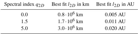
Table 1. The results for the two-dimensional bendover scalel2D
obtained for different values of the energy range spectral indexq2D.
The results were obtained by comparing theoretical results with the observations presented in Dasso et al. (2007).
Spectral indexq2D Best fitl2Din km Best fitl2Din AU
0.0 0.8·106km 0.005 AU
1.5 1.7·106km 0.011 AU
5.0 3.0·106km 0.020 AU
2.7 Temporal correlation functions
In the following we calculate the (combined) single-point-two-time correlation function defined byE⊥(t ):=R⊥(x= 0,t ). The latter function is also known as Eulerian correlation function. We obtain the Eulerian correlations from Eqs. (10) and (11) by settingz=0 andρ=0 therein
E⊥slab(t )=8π
Z ∞
0
dkkgslab(kk)0slab(kk,t )
E2D⊥ (t )=2π
Z ∞
0
dk⊥g2D(k⊥)02D(k⊥,t ). (21) Such correlation functions were already calculated analyti-cally in Shalchi (2008b) for a constant spectrum in the energy range (qslab=q2D=0 in our notation). It is straightforward to extend those results for the spectra defined in Eqs. (8) and (9). In this case and for the NADT model the following ana-lytical forms can be found
E⊥slab(t )=4D(s,qslab)δBslab2
Z ∞
0
dx x
qslab
(1+x2)(s+qslab)/2
×cos(xvAt / lslab)e−ξ vAt / l2D (22)
0 0.5 1 1.5 2 2.5 3 3.5 4 4.5 5
x 106
−0.2 0 0.2 0.4 0.6 0.8 1 1.2
z in km
R⊥
/
δ
B
2
Fig. 2. Spatial correlations for two-dimensional modes for different values ofq2D. We compare theoretical results forq2D=0 with
l2D=0.8·106km (dotted line),q2D=1.5 withl2D=1.7·106km
(solid line), andq2D=5.0 withl2D=3.0·106km (dashed line)
with the observations (black dots) from Dasso et al. (2007).
and
E2D⊥ (t )=4D(s,q2D)δB2D2
Z ∞
0
dx x
q2D
(1+x2)(s+q2D)/2
×e−ξ(1+x2)1/3vAt / l2D. (23) Here we have used again the integral transformations x=
kklslab and x=k⊥l2D, respectively. Furthermore we have used the parameterξ=
√
2δB2D/B0. In Sect. 3.2 we evalu-ate Eqs. (22) and (23) numerically and compare our findings with spacecraft data.
3 Comparison with spacecraft data
3.1 Spatial correlation functions
For slab modes we calculate spatial correlations fors=5/3 andqslab=0 and compare the result with the observations obtained by Dasso et al. (2007). These observations were obtained for the fast solar wind2 (VSW>470 km/s). Dasso et al. (2007) (see Fig. 2 for the case 0oof their paper) found for the spatial correlations along the mean magnetic field that
R⊥(z=380000km)≈0.4 AU. In Fig. 1 we fit Eq. (12) to the observations. We obtain the best fit forlslab≈0.6·106km= 0.004 AU3. We like to emphasize thatlslab is the slab ben-dover scale and not the correlation length. Furthermore, this fit is only correct if we indeed haveqslab=0.
2It was shown (for instance in Dasso et al., 2005) that the
struc-ture of the correlation function can differ for fast and slow solar wind.
3Here we used Astronomical Units (AU) which is approximately
0 0.2 0.4 0.6 0.8 1 0.7
0.75 0.8 0.85 0.9 0.95 1
Time in hours
E⊥
/
δ
B
2
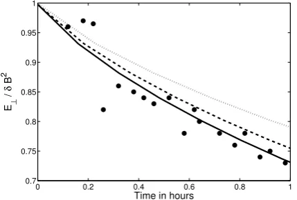
Fig. 3. The two-dimensional Eulerian correlation function as a function of the time. The observations (represented by the dots) are from Matthaeus et al. (2010) and the theoretical results were
computed by using Eq. (23). For the three theoretical results
we assumed thatδB2D=
√
0.8B0, q2D=1.5,vA=12 km/s, and
s=5/3. We used different values for the bendover scale of the two-dimensional modes, namelyl2D=1.0·106km (dotted line),
l2D=0.8·106km (dashed line), andl2D=0.7·106km (sold line). In Fig. 2 we determine the two-dimensional bendover scalel2D. In this case it is not clear what the energy range spectral index is (e.g. Matthaeus et al., 2007). Thus, we have calculated spatial correlations fors=5/3 and for different values ofq2D. For a different energy range spectral index we get the best agreement with the observations for a different bendover scale. Therefore, what we get forl2D depends on what we assume forq2D. In Table 1 the different parameter couples are listed. For instance we find the best agreement between theory and observations forl2D≈1.7·106km cor-responding to 0.011 AU if we setq2D=1.5.
3.2 Temporal correlation functions
Here we compare temporal or Eulerian correlations. As an approximation we assume pure two-dimensional turbulence4 and setξ =1.265. Furthermore we use again s=5/3 for the inertial range spectral index and for the Alfv´en speed we assumevA=12 km/s. In Figs. 3 and 4 we have shown a com-parison between the observations (Matthaeus et al., 2010) and the results obtained by evaluating Eq. (23) numerically. We have computed the temporal correlation functions for dif-ferent values of the two-dimensional bendover scalel2D and the energy range spectral indexq2D. It should be emphasized that the parameterl2D is the bendover scale used in Eq. (9) and not the correlation length. As shown in Figs. 3 and 4 we can reproduce the measured temporal correlations. There-fore, we conclude that the observations are consistent with our understanding of the turbulence dynamics.
4Here we assume pure two-dimensional turbulence as
approxi-mation because two-dimensional modes are dominant in the solar wind (Bieber et al., 1996). In the fast solar wind, however, there is a significant slab contribution.
0 0.2 0.4 0.6 0.8 1
0.65 0.7 0.75 0.8 0.85 0.9 0.95 1
Time in hours
E⊥
/
δ
B
2
Fig. 4. The two-dimensional Eulerian correlation function as a function of the time. The observations (represented by the dots) are from Matthaeus et al. (2010) and the theoretical results were computed by using Eq. (23). For the three theoretical results we
assumed thatδB2D=
√
0.8B0,l2D=0.7·106km,vA=12 km/s,
ands=5/3. We used different values for the energy range spectral index, namelyq2D=0.0 (dotted line),q2D=1.5 (solid line), and
q2D=5.0 (dashed line).
4 Conclusions
In the present paper we have compared analytical forms for correlation functions based on the work of Shalchi (2008a,b) with spacecraft measurements performed in the solar sys-tem for the fast solar wind by using the Advanced Compo-sition Explorer and the Wind spacecraft (e.g. Dasso et al., 2007; Matthaeus et al., 2010). Based on this comparison we found values for the bendover scales of the slab modes and the two-dimensional modes, respectively. For the slab ben-dover scale we find the best agreement forlslab≈0.6·106km
=0.004 AU. For the two-dimensional modes our findings for the bendover scale depends on the assumption of the energy range spectral index q2D - see Table 1 of the present pa-per. Forq2D=0.0 for instance we get the best fit by setting
l2D≈0.8·106km=0.005 AU. Forq2D=1.5, however, we obtainl2D≈1.7·106km=0.011 AU. It seems that the two bendover scales are in the same order of magnitude. The val-ues obtained in the present paper are close to those obtained by Dasso et al. (2007).
We have also compared analytical results for the tempo-ral or Eulerian correlation function with the observations ob-tained by Matthaeus et al. (2010). In this case we have ap-proximated the turbulence by using two-dimensional modes which are dominant in the solar wind5 (see Bieber et al., 1996). This comparison is shown in Figs. 3 and 4. As shown the two-dimensional bendover scale l2D as well as the en-ergy range spectral indexq2D have an influence on the Eu-lerian correlations. Forq2D=1.5 for instance, we find the best agreement if the bendover scale is l2D≈0.7·106km 5There are indications that there is a significant slab contribution
=0.004 AU. For other values ofq2D we would find the best agreement for a different bendover scale. Obviously the the-oretical correlation function for these cases agrees very well with the data points. Our results are summarized in Table 1.
In the current paper we have compared spatial and tem-poral correlation functions obtained analytically with solar wind observations. By fitting turbulence parameters we ob-tained a good agreement between theory and observations. We have shown that critical parameters are the bendover scaleslslab andl2D as well as the energy range spectral in-dex of the two-dimensional modesq2D. The results of the current paper show that the observations are consistent with our present understanding of solar wind turbulence which is based on the two-component model.
Acknowledgement. A. Shalchi acknowledges support by the
Natural Sciences and Engineering Research Council (NSERC) of Canada.
Edited by: T. Laitinen
Reviewed by: two anonymous referees
References
Batchelor, G. K.: Theory of Homogeneous Turbulence, Cambridge, 1970.
Bieber, J. W., Matthaeus, W. H., Smith, C. W., Wanner, W., Kallen-rode, M.-B., and Wibberenz, G.: Proton and electron mean free paths: The Palmer consensus revisited, Astrophys. J., 420, 294, 1994.
Bieber, J. W., Wanner, W., and Matthaeus, W. H.: Dominant two-dimensional solar wind turbulence with implications for cosmic ray transport, J. Geophys. Res., 101, 2511, 1996.
Dasso, S., Milano, L. J., Matthaeus, W. H., and Smith, C. W.: Anisotropy in Fast and Slow Solar Wind Fluctuations, Astro-phys. J., 635, L181, 2005.
Dasso, S., Matthaeus, W. H., Weygand, J. M., Chuychai, P., Mi-lano, L. J., Smith, C. W., and Kivelson, M. G.: ACE/Wind multi-spacecraft analysis of the magnetic correlation in the solar wind, ICRC, 2007.
Goldreich, P. and Sridhar, S.: Toward a theory of interstellar tur-bulence. 2: Strong alfvenic turbulence, Astrophys. J., 438, 763, 1995.
Hunana, P. and Zank, G. P.: Inhomogeneous Nearly Incompress-ible Description of Magnetohydrodynamic Turbulence, Astro-phys. J., 718, 148, 2010.
Matthaeus, W. H. and Smith, C.: Structure of correlation tensors in homogeneous anisotropic turbulence, Phys. Rev. A - General Physics, 24, 2135, 1981.
Matthaeus, W. H. and Goldstein, M. L.: Stationarity of magnetohy-drodynamic fluctuations in the solar wind, J. Geophys. Res., 87, 10347, 1982.
Matthaeus, W. H., Goldstein, M. L., and Roberts, D. A.: Evidence for the presence of quasi-two-dimensional nearly incompressible fluctuations in the solar wind, J. Geophys. Res., 95, 20673, 1990. Matthaeus, W. H., Dasso, S., Weygand, J. M., Milano, L. J., Smith, C. W., and Kivelson, M. G.: Spatial Correlation of Solar-Wind Turbulence from Two-Point Measurements, Phys. Rev. Lett., 95, 23, 2005.
Matthaeus, W. H., Bieber, J. W., Ruffolo, D., Chuychai, P., and Minnie, J.: Spectral Properties and Length Scales of Two-dimensional Magnetic Field Models, Astrophys. J., 667, 956, 2007.
Matthaeus, W. H., Dasso, S., Weygand, J. M., Kivelson, M. G., and Osman, K. T.: Eulerian Decorrelation of Fluctuations in the Interplanetary Magnetic Field, Astrophys. J. Letters, 721, L10, 2010.
Matthaeus, W. H., Servidio, S., Dmitruk, P., Carbone, V., Oughton, S., Wan, M., and Osman, K. T.: Local Anisotropy, Higher Order Statistics, and Turbulence Spectra, Astrophys. J., 750, 103, 2012.
Oughton, S., Priest, E., and Matthaeus, W. H.: The influence of a mean magnetic field on three-dimensional magnetohydrody-namic turbulence, J. Fluid Mech., 280, 95, 1994.
Oughton, S., Dmitruk, P., and Matthaeus, W. H.: A two-component phenomenology for homogeneous magnetohydrodynamic turbu-lence, Physics of Plasmas, 13, 042306, 2006.
Ruiz, M. E., Dasso, S., Matthaeus, W. H., Marsch, E., and Wey-gand, J. M.: Aging of anisotropy of solar wind magnetic fluctu-ations in the inner heliosphere, J. Geophys. Res., 116, A10102, 2011.
Shalchi, A., Bieber, J. W., Matthaeus, W. H., and Schlickeiser, R.: Parallel and Perpendicular Transport of Heliospheric Cosmic Rays in an Improved Dynamical Turbulence Model, Astrophys. J., 642, 230, 2006.
Shalchi, A., Tautz, R. C., and Schlickeiser, R.: Field line wandering and perpendicular scattering of charged particles in Alfv´enic slab turbulence, Astron. Astrophys., 475, 415, 2007.
Shalchi, A.: Analytical forms of correlation functions and length scales of astrophysical turbulence, Astrophys. Space Science, 315, 31, 2008a.
Shalchi, A.: Forms of Eulerian correlation functions in the solar wind, Astrophys. Space Science, 318, 149, 2008b.
Shalchi, A.: Nonlinear Cosmic Ray Diffusion Theories, Astro-physics and Space Science Library, Berlin, Springer, 362, 2009. Shalchi, A. and Weinhorst, B.: Random walk of magnetic field
lines: Subdiffusive, diffusive, and superdiffusive regimes, Adv. Space Res., 43, 1429, 2009.
Shalchi, A., B¨usching, I., Lazarian, A., and Schlickeiser, R.: Per-pendicular Diffusion of Cosmic Rays for a Goldreich-Sridhar Spectrum, Astrophys. J., 725, 2117, 2010.
Shalchi, A., Dosch, A., Le Roux, J. A., Webb, G. M., and Zank, G. P.: Magnetic-field-line random walk in turbulence: A two-point correlation function description, Phys. Rev. E, 85, 026411, 2012.
Shebalin, J. V., Matthaeus, W. H., and Montgomery, D.: Anisotropy in MHD turbulence due to a mean magnetic field, J. Plasma Phys., 29, 525, 1983.
Tu, C.-Y. and Marsch, E.: A model of solar wind fluctuations with two components - Alfv´en waves and convective structures, J. Geophys. Res., 98, 1257, 1993.
Weinhorst, B. and Shalchi, A.: Reproducing spacecraft measure-ments of magnetic correlations in the solar wind, Month. Not. Roy. Astronom. Soc., 403, 287, 2010.