Formal Verification of Secure Information Flow
in
Cloud Computing
Wen Zeng1 Maciej Koutny1 Paul Watson1 Vasileios Germanos2
1School of Computing Science, Newcastle University, Newcastle upon Tyne,
UK
e-mail: [email protected], {maciej.koutny, paul.watson}@ncl.ac.uk
2Department of Mathematics and Computer Science, Liverpool Hope
University, Liverpool, UK e-mail: [email protected]
Abstract
Federated cloud systems increase the reliability and reduce the cost of com-putational support to an organization. However, the resulting combination of secure private clouds and less secure public clouds impacts on the over-all security of the system as applications need to be located within different clouds. In this paper, the entities of a federated cloud system as well as the clouds are assigned security levels of a given security lattice. Then a dynamic flow sensitive security model for a federated cloud system is introduced within which the Bell-LaPadula rules and cloud security rule can be captured. The rest of the paper demonstrates how Petri nets and the associated verifica-tion techniques could be used to analyze the security of informaverifica-tion flow in federated cloud systems.
1. Introduction
The extent and importance of cloud computing is rapidly increasing due to the ever increasing demand for internet services and communications. Instead of building individual information technology infrastructure to host databases or software, a third party can host them in its large server clouds. However, large organizations may wish to keep sensitive information on their more restricted servers rather than in the public cloud. This has led to the introduction of federated cloud computing (FCC) in which both public and private cloud computing resources are used, see Watson (2012).
A federated cloud is the deployment and management of multiple cloud computing services with the aim of matching business needs. Data, ser-vices, and software are required to be allocated in different clouds for both security and business concerns. Although federated cloud systems (FCSs) can increase the reliability and reduce the cost of computational support to an organization, the large number of services and data on a cloud system creates security risks due to the dynamic movement of the entities between the clouds. As a result, it is necessary to develop tractable formal models faithfully capturing information flow security within FCSs.
2. Related Work
There exist different methods for addressing workflow1security; for
exam-ple, the flow-sensitive analysis of programs in Smith (2001) and Russo et al. (2009). Using Petri nets to model workflows, Knorr (2000, 2001) applied the Bell-LaPadula model to workflow security. In particular, Knorr (2000) considered theread and write security policies. In Knorr (2001), the deploy-ment of blocks within a workflow across a set of computational resources was not considered. In addition, the paper considered theclearance level but not
location level in its embodiment of Bell-LaPadula model.
Watson (2012) proposed to partition workflows over a set of available clouds in such a way that security requirements are met. The approach is based on a multi-level security model that extends Bell-LaPadula to encom-pass cloud computing. Watson (2012) also indicated that workflow transfor-mations are needed when data are communicated between clouds. However, in this study, the concurrency of the events or the execution of tasks in the system, the dynamic movement of the services, and the changes of the clearance level were not considered. Zeng et al. (2014b,a) introduced a flow sensitive security model to capture information flow in FCSs systems, which can be captured by CPNs. However, the clouds and services were assumed to be fixed, and the dynamic movement of services was not considered. Zeng and Koutny (2014) proposed a formal model for data resources in a dynamic environment focused on the location of different classes of data resources and users. However, the Bell-LaPadula rules and server-side components were not considered.
As far as we aware, there is limited work related to formal verification of security in cloud computing systems. As an example, Gouglidis and Mavridis (2013) proposed a methodology for the development and verification of access control systems in cloud computing. The authors verify the access control systems against organizational security requirements using techniques that are based on simple transition systems. As another example, Benzadri et al. (2014) employed Bigraphical Reaction Systems to formally specify cloud ser-vices and customers as well as their interaction schemes. However, they did not consider security policies.
1Information flow refers to paths followed by data from their original positions to
3. Security Policies in Cloud Computing Systems
In this section, we recall some basic concepts concerning security policies in cloud computing systems.
3.1. Information Lattices
Throughout the paper, we will assume that the basis of a federated cloud is a set P of single deployment clouds. Moreover, S will denote subjects (e.g., services, programs and processes), and O will denote objects (e.g., data resources and messages). Subjects and objects will jointly be referred to as entities, and their set will be denoted by E.
We will assign a security level to any entity, which will in practice be related to the degree of security of its contents, as well as to any cloud which will be related to the maximal security level of the entities it can contain.
A lattice for security concerns, Lsec = (Lsec,≤sec) consists of a set Lsec
and a partial order relation ≤sec such that, for all l, l0 ∈ Lsec, there exists a
least upper bound ltl0 ∈Lsec, and a greatest lower bound lul0 ∈Lsec. The
lattice is complete if each subsetLof Lsec has both a least upper bound `
L and a greatest lower bound Q
L, see Denning and Dorothy (1976), Denning and Dorothy (1982), and Landauer and Redmond (1993). Following Lan-dauer and Redmond (1993), we will assume that the security lattice Lsec is
complete.
3.2. Security Requirements: Bell-LaPadula
We adopt the Bell-LaPadula multi-level control model of Bell and La-padula (1973), with services modelled as the subjects S, and data as the objects O, Knorr (2001). Such a security model consists of the following components:
- A set of possible access rightsR. The commonly used access rights are
read (=r) and write (=w). In addition to reading and writing, there can be other access rights, e.g., data items that can be executed and/or updated. In order to simplify the presentation, the access rights used in this paper are read and write, R={r, w}.
- A complete lattice for security concerns,Lsec = (Lsec,≤sec) .
reads a data itemd0, then there will be the following entry in the access
control matrix: (s1, d0) 7→ {r, . . .}. Similarly, if a service s3 writes a
data item d2, then there will be the following entry in the matrix:
(s3, d2) 7→ {w, . . .}. Note that the empty set is a valid function value,
e.g., (s9, d7)7→ ∅ means that the subject s9 has no access rights to the
data item d7.
- A clearance map: c:S →Lsec. This represents the maximum security
level at which each subject (i.e., service) can operate.
- A security level map: ` : E → Lsec. This represents the security level
of each subject and object.
The Bell-LaPadula model states that a system is secure with respect to the above model if the following conditions are satisfied for all subjectss∈S and objects o∈O:
clearance: `(s)≤sec c(s) (1)
no-read-up: r ∈B(s, o)⇒c(s)≥sec `(o) (2)
no-write-down: w∈B(s, o)⇒`(o)≥sec `(s) (3)
For workflows, the implications of these conditions are that a subject: (i) can only operate at a security level that is less than or equal to its clearance; (ii) cannot read data that is at a higher security level than its own clearance; and (iii) cannot write data residing at a lower security level.
In the standard Bell-LaPadula model recalled above, it is implicitly as-sumed that the security levels of entities are fixed. However, in a typical FCS security scenario, the system moves through a set of states where these can change. We will deal with such a dynamic scenario in the rest of this paper. As a first step, we extend the Bell-LaPadula model by assigning security levels also to clouds:
- ` :E∪P →Lsec
Moreover, a new mapping loc is used to return the location of each entity: - loc:E →P
Then add an additional rule that an entity can only be deployed in a cloud with a security level that is greater than or equal to that of the entity. That is, for each entity e: an entity e is located in cloud p, then we must have
4. System Model
We now introduce a formal model for capturing the dynamic behaviour of federated cloud computing systems. Such a model can then be analyzed to verify that the system satisfies the requirements of a given set of Bell-LaPadula rules, as well as the cloud security rule for confidentiality consid-erations and any user-specified policies.
The proposed model uses tuples to represent entities located in the clouds. Each such tuple comprises information about the nature of the entity (ser-vice or data), the security information (the security and clearance levels), and the location information (the hosting cloud). Since there can be dupli-cates of both services and data within a given cloud, the state of the system is a multiset of entities, allowing for an arbitrary multiplicity of any ser-vice or object. The transformations of the system are then defined through the simultaneous execution of individual actions, each action being executed instantaneously and possibly many times.
It is assumed that the system is based on a fixed set of clouds with fixed security levels (issues involved in the modelling of dynamic changes of the set of clouds as well as their security levels are discussed in Remark 4.1). It is, however, possible to model the dynamic changes of the security levels of subjects and objects as well as their creation and destruction.
To aid the understanding of the system model, it is introduced in three stages. First, we specify the overall structure in Definition 1. Then, in Definition 2, we introduce rules which explain the dynamic transformation between the system states. Finally, in Sections 4.1, 4.2, and 4.3, we specify the exact format of the three kinds of actions supported by the model. Definition 1 (Dfssm structure). A dynamic flow-sensitive security model
for federated clouds is a septuple:
DFSSM = (P, S, O,Lsec, `,A, stinit), (5)
where: P is a finite nonempty set of clouds; S is a finite nonempty set of subjects/services; O is a finite nonempty set of objects/data; Lsec is a
complete security lattice; ` :P → Lsec is a mapping assigning security levels
to the clouds; A=Aac] Adf ] Acf is a finite set of actions, each action being
a pair φ= (φin, φout) consisting of two finite multisets over the set of tuples
and stinit is an initial state defined as a finite multiset over M. In general,
a state of DFSSM is a finite multiset over M, and x∈ M is present in a state st if st(x)>0.
A tuple (s, l, c, p)∈ M, denoted by (s, l, c)@p, represents a service swith the security level l and the clearance level c (c ≥sec l) residing on cloud p.
Similarly, a tuple (o, l, p) ∈ M, denoted by (o, l)@p, represents a data item o with the security levell residing on cloudp.
An entity can have several different copies, and each of these copies can have a different security level and may reside in a different cloud. As already mentioned, we allow multiple copies of a single entity to be present in a cloud. Hence a state is a multisetstoverMrather than a subset ofM. For example,st8(s6,1,2, p4) = 4 means that in the statest8 there are four copies
of service s6 with security level 1 and clearance level 2 residing on cloudp4.
Now we define how the system can proceed from one state to another state by executing a multiset of actions. It is assumed that the executed (instances of) actions cannot share input entities. For example, if there is one copy of an entity present, then at most one action which has this entity in its input can be executed. This results in conflicts between actions which could potentially be executed, and contributes to nondeterminism in system execution. The formal semantics, and then property verification, take into account all possible ways in which such conflicts could be resolved.
Below (−) and (+) are respectively the multiset subtraction and addition operations.
Definition 2 (Dfssm semantics). A multiset Φ = {φ1, . . . , φn} of actions
over A, where φi = (φini , φiout) for i= 1, . . . , n, is enabled at state st if
Φin =φin1 +. . .+φinn ≤st .
Then Φ can then be executed leading to a state st0 given by:
st0 =st−Φin+ Φout =st−Φin +φout1 +. . .+φoutn .
We denote this by st−→Φ st0.
With such a definition we can state precisely what are the states which can be reached from the initial one.
Definition 3 (Dfssm reachable states). The reachable states of DFSSM in Definition 1 is the minimal set of states RS containing stinit such that if
Dfssmis intended to model a federated cloud system that is divided into
three sub-models: the access control sub-system, the data flow sub-system, and the control flow sub-system. To reflect this division, we will now describe the format of action sets employed by these three sub-models: Aac (for access
control), Adf (for data flow), and Acf (for control flow).
4.1. Access Control Sub-system
To simplify the presentation, we will assume that a subject can only access a single object at a time. Then, in the access control sub-system, each φ = (φin, φout)∈ A
ac is such that:
φin = {(s, l, c)@p,(o, l0)@p} or φin = {(s, l, c)@p} φout = {(s0, l, c)@p,(o0, l00)@p} or φout = {(s0, l, c)@p}
where p∈ P, s, s0 ∈ S, o, o0 ∈O, and l, l0, l00, c ∈Lsec. Moreover, as we need
to formally capture the security policy of the cloud system, the set of actions Aac is composed of two subsets: the read actions A
(r)
ac, and write actions
A(acw).
The basic form of a read action is:
φin = {(s, l, c)@p,(o, l0)@p} and φout = {(s0, l, c)@p,(o, l0)@p}
where
c≥sec l0 & `(p)≥sec cul0 (6)
according to the Bell-LaPadula rules (1,2) and the cloud security rule (4). Moreover, to represent destruction of objects, we allow destructive read ac-tions of the form:
φin = {(s, l, c)@p,(o, l0)@p} and φout = {(s0, l, c)@p}
where, as before, c≥sec l0 and `(p)≥sec cul0.
The basic form of a write action is:
φin = {(s, l, c)@p,(o, l0)@p} and φout = {(s0, l, c)@p,(o0, l00)@p}
where
l00≥sec l & `(p)≥sec cul0ul00 (7)
according to the Bell-LaPadula rules (1,3) and the cloud security rule (4). Moreover, to represent the creation of objects, we allow creation actions of the form:
φin = {(s, l, c)@p} and φout = {(s0, l, c)@p,(o0, l0)@p}
4.2. Data Flow Sub-system
Objects can migrate between different clouds. Each actionφ= (φin, φout)∈
Adf is such that:
φin = {(o, l)@p} and φout = {(o0, l0)@p0},
(8) where p, p0 ∈P, o, o0 ∈O, and l, l0 ∈Lsec.
4.3. Control Flow Sub-system
Similarly, services can also migrate between different clouds. The last type of actions concerns the migration of the subjects in different locations. Each action φ= (φin, φout)∈ A
cf is such that:
φin = {(s, l, c)@p} and φout = {(s0, l0, c0)@p0}, (9)
where p, p0 ∈P, s, s0 ∈S, and l, l0, c, c0 ∈Lsec.
Note also that in practice the actions in A can be specified in a more convenient way; for example, by using guards and parameters. This is illus-trated in the Petri net representation discussed later in this paper, where net transitions use guards and arcs use parameters (variables).
Remark 4.1. The system model introduced above has been kept deliberately simple, or low-level. This should allow one to define on top of it a variety of user-friendly, and thus more practical, notations for system specification and property verification. We will demonstrate in the rest of this paper how this can be achieved.
Despite its relative simplicity, the model is very expressive and yet tractable. Basically, it is equivalent to the model of Place/Transition nets (PTNs) in-troduced in Section 5 which is a class of Petri nets where state reachability is decidable (it is generally accepted that PTNs are a fundamental class of concurrent system models where reachability is decidable).
conjecture that allowing dynamic creation and deletion of clouds as well as changing of their security levels would also lead to a Turing powerful model. Therefore, as one of our aims is to keep the system model tractable, we believe that the formalisation presented above strikes a right balance between being useful for practical applications and amenable to automated verification.
4.4. System Security
We now can capture a key property of information flow across different clouds.
Definition 4. Let DFSSM be as in (5). A state st of DFSSM is secure if
`(p) ≥sec l and `(p)≥sec c, for all entities (o, l)@p and (s, l, c)@p present in
st. Moreover, DFSSM is secure if all its reachable states are secure.
That is, a state is secure if all copies of entities present reside in clouds without causing security violation. One can then state a general security policy guaranteeing the security of the system model. Such a policy is for-mulated by placing a suitable condition on the actions of the model.
Theorem 4.1. Let DFSSM be as in (5) and the following hold:
- l0 ≤sec `(p0), for every action φ ∈ Adf as in (8), and
- l0 ≤sec c0 ≤sec `(p0), for every action φ∈ Acf as in (9).
Then DFSSM is secure provided that stinit is secure.
The above result can only be applied in specific cases, e.g., when the sys-tem applies very strict security policies to the migration of data and services. In general, we need to verify that a given system specification yields a secure system, e.g., by applying a suitable model checking technique.
4.5. Well-formedness
In addition to verifying the security property of Definition 4, there are other desirable functional properties which one would normally need to ver-ify using, e.g., model checking tools. The following are examples of such properties formulated for DFSSM in (5):
- DFSSM isbounded, if there isn≥1 such that the size of each reachable state is less than n.
- DFSSM iswell-formed, if there is a state stsuch thatDFSSM is both live and bounded after replacing stinit by st.
5. Petri Nets
Petri nets are a graphical modelling tool for a formal description of sys-tems whose dynamics are characterized by concurrency, synchronization, mu-tual exclusion and conflict. In this section, we briefly recall three classes of Petri nets used in our discussion (see Reisig (1985) and Jensen (2009) for more details).
5.1. Place/Transition Nets
A Place/Transition net (PTN) N consists of two disjoint finite sets of nodes, P l and T r, respectively calledplaces and transitions, a mapping W : (P l×T r)∪(T r×P l)→ N specifying the weights of arcs that connect the nodes, and the initial marking (state) M0 : P l → N. In general, any finite
multiset of places is a marking (or state) of N.
Intuitively, places carry (black) tokens which represent the current dis-tribution of resources in a system modelled by the net. In other words, the current state of the modelled system is given by the number of tokens in each place.
Transitions are the active components of the net. An input arc of a transitiontrstarts at a placepland ends attrprovided thatn=W(pl, tr)> 0. In such a case, n is the arc’s weight signifying that an execution of tr requires n tokens in pl which are consumed as a result. Similarly, an output arc from tr to pl exists provided that m = W(tr, pl)> 0, and an execution of tr inserts m tokens into pl.
A transition tr is allowed to be executed (or fired) at a marking M if M(pl) ≥ W(pl, tr), for all places pl. Its firing produces a new marking M0 such thatM0(pl) =M(pl)−W(pl, tr)+W(tr, pl), for all placespl. In general, one can fire a finite multiset of transitions U ={tr1, . . . , trk} provided that
M(pl)≥W(pl, tr1) +· · ·+W(pl, trk), for all places pl (that is, input tokens
cannot be shared), and its firing results in a markingM0 such thatM0(pl) = M(pl) − W(pl, tr1) − · · · − W(pl, trk) + W(tr1, pl) + · · · +W(trk, pl), for
starting from the initial marking, and introduce the notion of a reachable marking.
Petri nets, in particular PTNs, have been widely used for structural mod-elling of workflows and have been applied in a wide range of qualitative and quantitative analyzes (see, for example, van der Aalst (1996, 1997, 1998)). A Petri net representing a workflow has, in particular, the following charac-teristics:
- Workflow activities are represented by net transitions, and executing an activity corresponds to the firing of a transition.
- Net markings represent the states of the corresponding workflow. Each token represents a control flow point of one of the concurrent processes described by the workflow, or an existing data resource.
5.2. Coloured Petri Nets
PTNs are a low-level model, and in practical applications, it is conve-nient to use more compact (but behaviourally equivalent) high-level Petri net models. An example of such a compact model are coloured Petri nets
(CPNs), where the tokens are tuples of values, the arcs are used as selectors allowing one to specify the format of input and output tokens, and transi-tions have associated guards which allow one to easily express, e.g., various security policies.
Let Tok be a finite set of elements (or colours) and VAR be a disjoint finite set of variable names. In a CPN:
- Each place has a type, which is a subset of Tok indicating the colour of tokens this place can contain. A marking is obtained by placing in each place a multiset of tokens belonging to the type of the place. - Each arc is labelled with a multiset of variables fromVAR.
- Each transition has aguard, which is a Boolean expression over Tok∪
VAR. For a transition t, VAR(t) denotes the set of variables appearing in its guard and labelling its input and output arcs.
If this mapping can be extended to a total mappingσ0 in such a way that the guard of t evaluates to true and the values of the variables on the outgoing arcs are consistent with the types of the places these arcs point to, then t is
enabled and σ0 is an enabling binding of t. An enabled transition can fire, consuming the tokens from its pre-set and producing tokens in places in its post-set, in accordance with the values of the variables on the appropriate arcs given by σ0. One can then define an enabling condition and firing rule for a multiset of transitions with enabling bindings similarly as it was done for PTNs, and introduce notions like marking reachability by generalizing those defined for PTNs.
5.3. Labelled Petri Nets
The class we need allows one to describe properties related toobservability
of executed transitions.
A labelled Petri net (LPN) is a triple N =(N, X, lab) such thatN is an unlabelled net; Xis a finite set of labels; andlab :T r →X∪{}is a labelling function, and is the empty word. The labelling function associates to each transition tr a label lab(tr) indicating how tr is observed by an external environment. In particular, lab(tr) =means that tr is invisible, orinternal
to the computing system represented by N.
6. Dynamic Flow-sensitive Security Model in CPNs
We will now outline how CPNs could be used to represent (and then used to verify) a given Dfssm. To facilitate the discussion, following the
definitions in Section 4, the net modelling Dfssm is decomposed into three
parts: theaccess control sub-net, data flow sub-net, andcontrol flow sub-net.
6.1. Access Control Sub-net
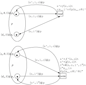
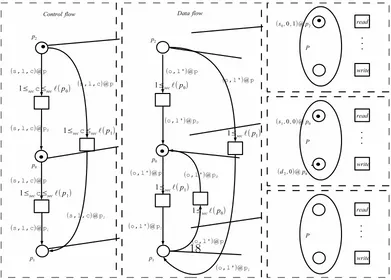
Figure 1: Basic structure of the access control sub-net. It shows one subject and one object, both residing on the same cloud,p2. Note thats,l, etc., are parameters (variables), and
services. Sincef, f0 are partial functions, they can be used to filter out pairs (s, o) for which there is no read and/or write access. Moreover, s0 = f(s,o) checks whether a service can read data or not, andl00 =h(s,o,l0,l00) specifies that after a service writes data, the security level of the data will be changed from l0 tol00, ando0 =g(s,o) specifies how the new data value is calculated.
6.2. Data Flow and Control Flow Sub-nets
We will now use an example to illustrate the definition of a dynamic flow-sensitive security model, and the way it can be represented using coloured Petri nets.
We consider two public clouds,p0 and p1, and one private cloud,p2. The
security levels of clouds, services, and data are listed in Table 1. As services and data can be deployed on different clouds, Table 2 shows all the valid mappings of entities to clouds. We can observe, e.g., that both s0 and s1
can be deployed on p0, p1, and p2. However, the data item d0 can only be
deployed on cloud p2.
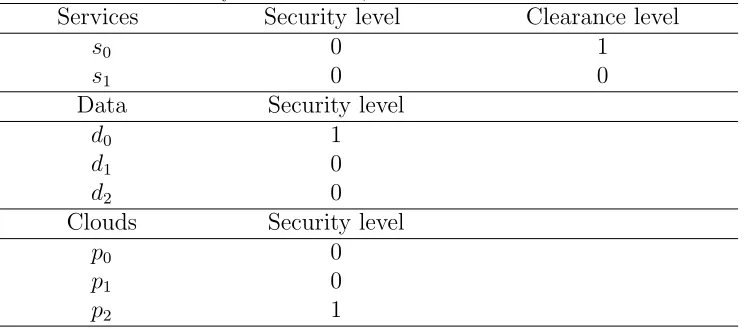
Table 1: Security level of clouds, services and data in the Dfssm.
Services Security level Clearance level
s0 0 1
s1 0 0
Data Security level
d0 1
d1 0
d2 0
Clouds Security level
p0 0
p1 0
p2 1
We assume that in the initial state of the system there is one data item, d0, and two services, s0 and s1, all residing on cloud p2. Moreover, in this
example we assume that the functions f, f0, g, h do not change the values associated with the entities except that g(s0, d0) =d1,h(s0, d0,0,1) = 0 and
g(s1, d1) =d2. That is, services0 can re-write the data item d0 into d1 and
reduce its security level to 0, whereas service s1 can re-writed1 into d2.
Table 2: Valid mappings of entities to clouds
Entities Cloudp0 Cloud p1 Cloud p2
s0 • • •
s1 • • •
d0 •
d1 • • •
d2 • • •
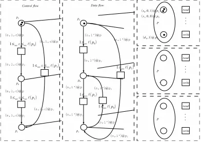
Figure 2: A Petri net model of a system consisting of cloudsp0,p1 andp2, as well as two
the right) is represented schematically (see Fig. 1 for its internal details). Note that places are labelled with the names of the corresponding clouds, and a dashed line joins two duplicate depictions of the same place.
The two servicess0 ands1 are represented by two tokens in place labelled
asp2in control flow, one token being (s0,0,1)@p2 and the other (s1,0,0)@p2.
The leftmost sub-net (control flow sub-net) shows how the services can grate between different clouds. Note that the security policy for service mi-gration is represented by the guards of the forml≤sec c≤sec `(p1) associated
with the transitions in the control flow sub-net (see Section 4.4).
The data resources are represented by a single token, (d0,1)@p2, inside
another place labelledp2 (belonging to thedata flow sub-net). It follows from
the security levels of the data resources and clouds that such a resource can never enter p0 or p1. Note also that the security policy for data migration
is represented by the guards of the form l ≤sec `(p0) associated with the
transitions in the data flow sub-net (see Section 4.4).
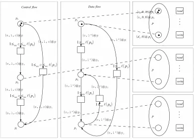
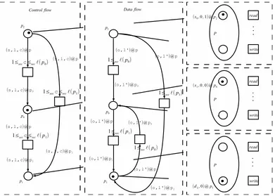
Figure 4: A reachable state of the system with s1 and d1 residing on cloud p0; and s0
residing on cloud p2.
Figure 6: A reachable state of the system with s1 residing on cloud p0; d2 residing on
cloudp1; and s0residing on cloud p2.
We can then illustrate the dynamic behaviour of the system modelled by CPN using a series of diagrams depicting four reachable states: (i) Fig. 3: after service s0 re-wrote d0 to d1 on cloud p2; (ii) Fig. 4: after service s1
and data d1 migrated from cloud p2 to cloudp0; (iii) Fig. 5: after service s1
re-wrote d1 tod2 on cloudp0; and (iv) Fig. 6: after datad2 migrated to cloud
p1.
the best of our knowledge, this is the first study of this kind.
7. Diagnosis and WF-diagnosability
In this section, we outline the diagnosis and weakly fair diagnosability property. This formal verification technique will be used in Section 8.
Diagnosis is the procedure of discovering abnormal behaviours of a sys-tem, and diagnosability is an associated property of, e.g., a Petri net stating that in any possible execution sequence (called below executions) an occur-rence of a fault can eventually be diagnosed. Sampath et al. (1995) proposed a method for diagnosability based on the construction of adiagnoser automa-ton that allows one to estimate states of the system by observing executions. Subsequent improvements were introduced in Jiang et al. (2001) and Schu-mann and Pencol´e (2007), where the basic idea was to build a verifier by constructing the product of the system with itself through synchronisation on observable transitions. If the system is given as an LPN, then the verifier can be constructed directly (see Madalinski and Khomenko (2010)), and the problem reduces to model checking of a fixed property expressed in LTL-X (see Pnueli (1977) and Lamport (1983)). Subsequently, Haar et al. (2003) proposed the weak diagnosis which is in fact more powerful than the stan-dard diagnosis as in Benveniste et al. (2003). Based on the weak diagnosis, the weakly fair diagnosability verification property was proposed in Agarwal et al. (2012) and then improved in Germanos et al. (2014).
7.1. Petri Nets and Diagnosability
The system under consideration is modelled by an LPN N. Transitions are partitioned into observable and invisible, i.e., the labelling function lab maps transitions toObs∪{ε}, whereObsis an alphabet ofobservable actions and ε /∈Obs is the empty word representing invisible action. This labelling function labcan be applied to finite and infinite executions, projecting them onto words in Obs∗ or Obsω. We assume that the N is free from deadlocks
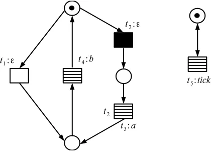
and divergencies, i.e., every execution can be extended to an infinite one, and every infinite execution has infinitely many observable transitions. Some of the invisible transitions are designated as faults. An example in Fig. 7 has observable transitions t3, t4, and t5 with lab(t3) = a, lab(t4) = b and
lab(t5) = tick (the other transitions are unobservable, i.e., invisible). Note
Figure 7: An undiagnosable LPN which would be diagnosable withoutt5. Makingt3 WF
makes the LPN diagnosable.
7.1.1. Standard diagnosability
Given a finite executionψ ofN, the observer seeslab(ψ)∈Obs∗, and only on this basis needs to conclude whether some fault transitiontr has occurred inψ. In a diagnosable system, once a fault has occurred, the observer is able toeventually detect this fact. That is, provided that the suffix ofψ after the first occurrence of a fault is sufficiently long, the observer should be able to conclude that each execution ρ with lab(ρ) = lab(ψ) involves a fault which has either already occurred or will definitely occur in future.
Definition 5 (Diagnosability). Nis diagnosableif for all infinite executions
ψ and ρ such that lab(ψ) =lab(ρ), ψ contains a fault iff ρ contains a fault.
For example, the LPN in Fig. 7 is not diagnosable. Indeed, one can only conclude that fault has occurred after observing a. However, the infinite execution t2tω5 contains a fault but never fires t3. If t5 is removed, the LPN
becomes diagnosable.
7.2. Weak Fairness
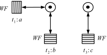
One can capture this idea using weak fairness (see Vogler (1995)). First, the designer specifies transitions which cannot be postponed indefinitely, des-ignating them as weakly fair (WF). An infinite execution ψ is then weakly fair (WF) if, for each WF transition tr, if tr is enabled after some prefix of ψ then the rest of ψ contains at least one transition in conf l(tr), where conf l(tr) is the set of all transitions tr0 6= tr sharing an input place with tr, see Fig. 8. Moreover, all finite executions are regarded as WF. One than takes the WF executions as a refined semantics of the net, i.e., other execu-tions are considered impossible. Coming back to the example in Fig. 7, if t3 is WF then the execution t2tω5 is not WF and thus disallowed, and so the
LPN becomes diagnosable.
Figure 8: (i) The execution (t1t2t3)ωis WF as no enabled transition is continually ignored
by it. (ii) The execution (t1t2)ω is not WF as t3 is enabled but all the transitions in
conf l(t3) ={t3} are continually ignored. (iii) The execution (t1t3)ω is WF: even though
t2is continually ignored, t1∈conf l(t2) ={t1, t2} is fired.
Definition 6(WF-diagnosability). Nis WF-diagnosableif each infinite WF execution ψ containing a fault has a finite prefix ψˆ such that every infinite WF execution ρ with lab( ˆψ)< lab(ρ) contains a fault.
The way of constructing a verifier corresponding to WF-diagnosability was described in Germanos et al. (2014). Using it, we can check the satis-faction of an LTL-X formula that captures the WF-diagnosability property.
8. Experimental Results
We now present experimental results relating to the diagnosis of potential actions of malicious insider in a cloud computing systems.
rules (1), (2), and (3). Instead, we evaluate the cloud security rule (4) which states that an entity must be deployed on a cloud with a security level that is greater than or equal to that of the entity. In other words, an entity can move to another cloud according to its security permission. We then assume that a malicious insider can move some entities to unauthorised clouds. This should, clearly, be detected and addressed by the cloud management system. For the verification task, we used theMariatoolset (see M¨akel¨a (2005)).
Its on-the-fly model checker verifies properties expressed in temporal logic by computing the product of a property automaton and the reachability graph of an LPN interpreted as automaton. Benchmark representations in Maria
input language are available from the authors upon request.
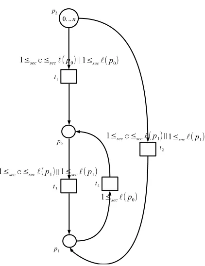
DfssmCloud (n#S, n#D). Fig. 9 shows an LPN modelling the system
comprising three clouds,p0,p1andp2. Cloudp2containsnservices (indicated
by (n#S)) and n data items (indicated by (n#D)). These entities can be distributed to clouds p0 and p1, according to some predefined security policy
respecting Dfssm, via transitions t1 and t3, respectively. Also, services and
data can flow from cloud p2 to cloud p1 directly via transition t2. It should
be noted that both services and data can flow from cloud p2 to clouds p0
and p1, and, similarly, from cloud p0 to cloud p1. However, from cloud p1 to
cloud p0 only data can flow. Thus, eventually, cloud p2 will become empty,
as only data can move from cloud p1 to cloud p0 and vice versa, and services
Figure 9: TheDfssmCloudbenchmark, which corresponds to the net in Fig. 2. The nets ofControl Flow andData flow are merged into a single net.
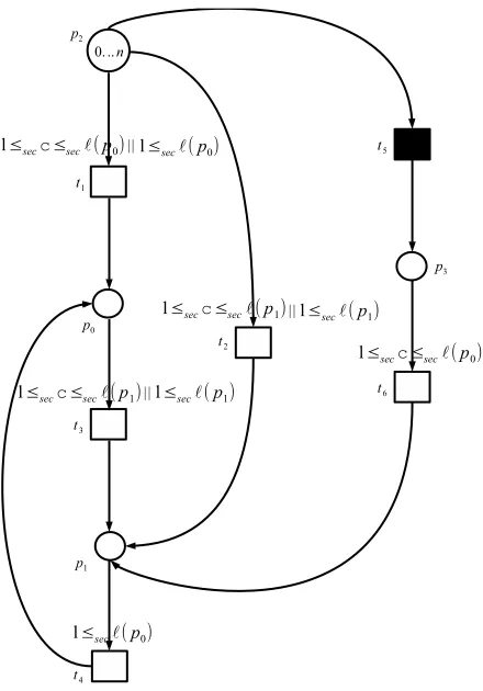
DfssmCloudIns(n#S, n#D). Fig. 10 shows the previous system with
a malicious insider represented by a black transition t5. The actions of the
insider are invisible and they can move services and data from cloud p2 to
p3. If this happens, then no entities will be moved from cloud p2 to cloud
p1 via cloud p0, or directly to cloud p1 via transition t2. Although cloud p3
can send entities to cloud p1, the type of entities it can send is restricted
to services. Thus, if an attack occurs, no data can be sent to cloud p0 as
it was expected, and it will finally remain empty. Moreover, even if the services can be transferred to cloud p1 from cloud p3, it is not guaranteed
that they have not been modified by the malicious insider, making the entities untrustworthy.
NoDfssmCloudIns (n#S, n#D). Fig. 11 is similar to Fig. 10 except
that it does not model aDfssm cloud system because we removed the
Figure 10: The DfssmCloudIns benchmark. The black transition indicates malicious behaviour in the system.
Initially, we verify that the security rule (4) holds in Fig. 9. The specific property for this case is captured by the LTL-X formula φ1 = ♦p0, i.e.,
data will always be sent to cloud p0. This is achieved by assigning security
guards in the transitions which allow specific entities to move to each cloud. The next case is to verify that the action of the malicious insider (see Fig. 10) can be detected due to the introduced dynamic flow-sensitive security policy. Here, we check again whether p0 will eventually contain some data
using the same LTL-X formula as previously. In this case, the formula is violated as it is possible for cloudp1 to contain only services and cloudp3 to
contain only data.
to detect the malicious action by applying diagnosis. To this end, we build a corresponding verifier (Fig. 11), as explained in Germanos et al. (2014), and check whether the WF-diagnosability property holds. It should be noted that in this model the transitions do not have guards to ensure that the security policy holds. Checking the WF-diagnosability property, the detection of a malicious insider becomes more ‘expensive’ in verification time. That is, each time the size of the model is increased, the state space of the verifier is increased significantly. We are therefore assured that a malicious action can be detected. In our case, we verify the following WF-diagnosability property
φdiag =p2∨♦¬ stub monitor
This property states that our cloud computing system is diagnosable, mean-ing that a malicious action can be detected, ifp2 is always marked or eventu-ally the place stub monitor is empty. This is necessary because if the faulty transition t05 fires, the WF stub transition will be enabled, and after firing the place stub monitor will become empty indicating the occurrence of a malicious action. Similarly, if transition t5 fires then the place p2 becomes
Figure 11: The NoDfssmCloudInsbenchmark (left) and the corresponding verifier (right). The black transition indicates malicious behaviour.
The experimental results are summarised in Tables 3, 4, and 5, where the meaning of the columns is as follows (from left to right): the name of a benchmark, the verification time, and the number of states. The time is measured in seconds. All experiments were conducted on a PC with 64-bit Windows 7 operating system, an Intel Core i7 2.8 GHz Processor with 8 cores and 4GB RAM (no parallelisation was used for the results in this table). The
Maria tool has confirmed that the verification property of each benchmark
Benchmarks Vrf Time Number of states
DfssmCloud (1#S, 1#D) 0.047 9
DfssmCloud (2#S, 2#D) 0.046 31
DfssmCloud (3#S, 3#D) 0.062 65
DfssmCloud (4#S, 4#D) 0.062 111
DfssmCloud (5#S, 5#D) 0.077 169
Table 3: Experimental results forDfssmCloudbenchmark.
Benchmarks Vrf Time Number of states
DfssmCloudIns(1#S, 1#D) 0.12 15
DfssmCloudIns(2#S, 2#D) 0.20 78
DfssmCloudIns(3#S, 3#D) 0.31 263
DfssmCloudIns(4#S, 4#D) 0.46 681
DfssmCloudIns(5#S, 5#D) 0.71 1479
Table 4: Experimental results forDfssmCloudInsbenchmark.
Benchmarks Vrf Time Number of states
NoDfssmCloudIns(1#S, 1#D) 0.11 315
NoDfssmCloudIns(2#S, 2#D) 1 2772
NoDfssmCloudIns(3#S, 3#D) 6 13500
NoDfssmCloudIns(4#S, 4#D) 39 47025
NoDfssmCloudIns(5#S, 5#D) 79 131859
Figure 12: Verification time increases dramatically when the number of services and data inNoDfssmCloudIns becomes larger. The verification times of DfssmCloudand
Df-ssmCloudIns are almost the same.
Figure 13: The state space increases dramatically when the number of services and data in NoDfssmCloudIns becomes larger. The state space of DfssmCloud and
Dfssm-CloudIns are almost the same.
benchmarks. We can observe that in a standard cloud system the verification of diagnosability increases significantly with the size of the system.
9. Conclusions
In this paper, we presented a dynamic flow-sensitive security model which can be used to analyze the information flow in FCSs. The entities present in the cloud system can be assigned different security levels belonging to a given security lattice. Moreover, each cloud is assigned a security level which captures the confidentiality level of the cloud. It is also possible to specify in a formal way different security policies for the movement of entities between different clouds. The resulting formal model can then be represented by a suitable CPN, and its dynamic behaviour analyzed using the existing verification methods and tools developed for Petri nets. We also discussed how diagnosability under weak fairness could be used to detect malicious intruders within an FCS.
10. Acknowledgments
We would like to thank the referees for their comments and useful sugges-tions. This research was supported by the 973 Program Grant 2010CB328102, NSFC Grant 61133001, and EPSRC UNCOVER project.
References
Agarwal, A., Madalinski, A., Haar, S., 2012. Effective verification of weak diagnosability. In: Proc. SAFEPROCESS’12. IFAC.
Bell, D. E., Lapadula, L. J., 1973. Secure Computer Systems: Mathematical Foundations. Tech. rep., MITRE Technical Report 2547.
Benveniste, A., Fabre, E., Haar, S., Jard, C., 2003. Diagnosis of asynchronous discrete event systems: a net unfolding approach. Automatic Control IEEE Transactions on 48 (5), 714–727.
Denning, R., Dorothy, E., May 1976. A lattice model of secure information flow. Commun. ACM 19, 236–243.
Denning, R., Dorothy, E., 1982. Cryptography and data security. Addison-Wesley Longman Publishing Co., Inc., Boston, MA, USA.
Germanos, V., Haar, S., Khomenko, V., Schwoon, S., 2014. Diagnosability Under Weak Fairness. In: Application of Concurrency to System Design (ACSD). pp. 132–141.
Germanos, V., Haar, S., Khomenko, V., Schwoon, S., 2015. Diagnosability Under Weak Fairness. ACM Trans. Embed. Comput. Syst. 14 (4), 1–19. Gouglidis, A., Mavridis, I., 2013. A Methodology for the Development and
Verification of Access Control Systems in Cloud Computing. In: Collabo-rative, Trusted and Privacy-Aware e/m-Services. Springer, pp. 88–99. Haar, S., Benveniste, A., Fabre, E., Jard, C., 2003. Partial Order
Diagnos-ability of Discrete Event Systems using Petri Nets Unfoldings. In: 42nd IEEE Conference on Decision and Control (CDC).
Jensen, K., 2009. Coloured Petri Nets. Springer Verlag Berlin Heidelberg. Jiang, S., Huang, Z., Chandra, V., Kumar, R., 2001. A polynomial algorithm
for testing diagnosability of discrete event systems. In: IEEE Trans. on Autom. Control.
Knorr, K., 2000. Dynamic Access Control Through Petri Net Workflows. In: Proceedings of the 16th Annual Computer Security Applications Confer-ence. ACSAC ’00. pp. 159–167.
Knorr, K., 2001. Multilevel Security and Information Flow in Petri Net Workflows. In: 9th International Conference on Telecommunication Systems -Modeling and Analysis, Special Session on Security Aspects of Telecom-munication Systems.
Lamport, L., 1983. What good is temporal logic? In: Proc. IFIP Congr.’83. Elsevier, pp. 657–668.
Madalinski, A., Khomenko, V., 2010. Diagnosability Verification with Par-allel LTL-X Model Checking Based on Petri Net Unfoldings. In: Proc. SysTol’10. pp. 398–403.
M¨akel¨a, M., 2005. maria: The Modular Reachability Analyzer. URL:
http://www.tcs.hut.fi/Software/maria/ index.en.html.
Pnueli, A., 1977. The Temporal Logic of Programs. In: Proc. FOCS’77. pp. 46–57.
Reisig, W., 1985. Petri nets: An Introduction. EATCS MONOGRAPHS. SPRINGER.
Russo, A., Sabelfeld, A., Chudnov, A., 2009. Tracking Information Flow in Dynamic Tree Structures. In: Proceedings of the 14th European Confer-ence on Research in Computer Security. ESORICS’09. Springer-Verlag, Berlin, Heidelberg, pp. 86–103.
Sampath, M., Sengupta, R., Lafortune, S., Sinnamohideen, K., Teneketzis, D., 1995. Diagnosability of Discrete Events Systems. IEEE Trans. on Au-tom. Control 40 (9), 1555–1575.
Schumann, A., Pencol´e, Y., 2007. Scalable diagnosability checking of event-driven systems. In: Proc. IJCAI’07. pp. 575–580.
Smith, G., 2001. A new type system for secure information flow. In: In CSFW14. IEEE Computer Society Press, pp. 115–125.
van der Aalst, W., 1996. Petri-net-based workflow management software. In: Proceedings of the NFS Workshop on Workflow and Process Automation in Information Systems. pp. 114–118.
van der Aalst, W., 1997. In: Application and Theory of Petri Nets 1997. Vol. 1248. pp. 407–426.
van der Aalst, W., 1998. The Application of Petri nets to Workflow Manage-ment. Journal of Circuits, Systems and Computers 08 (01), 21–66.
Watson, P., 2012. A multi-level security model for partitioning workflows over federated clouds. Journal of Cloud Computing 1 (1), 1–15.
Zeng, W., Koutny, M., 2014. Data Resources in Dynamic Environments. In: IEEE 8th International Symposium on Theoretical Aspects of Software Engineering (TASE). pp. 185–192.
Zeng, W., Koutny, M., Watson, P., 2014a. Verifying Secure Information Flow in Federated Clouds. In: IEEE 6th International Conference on Cloud Computing Technology and Science, CloudCom 2014, Singapore, Decem-ber 15-18, 2014. pp. 78–85.