High level synthesis FPGA implementation of the Jacobi algorithm to solve the Eigen problem

(1)

Research Article

High Level Synthesis FPGA Implementation of

the Jacobi Algorithm to Solve the Eigen Problem

Ignacio Bravo,

1

César Vázquez,

1

Alfredo Gardel,

1

José L. Lázaro,

1

and Esther Palomar

2

1_{Electronics Department, University of Alcal´a, Alcal´a de Henares, 28805 Madrid, Spain}

2_{School of Computing, Telecommunications and Networks, Birmingham City University, Millennium Point, Birmingham B4 7XG, UK} Correspondence should be addressed to Ignacio Bravo; [email protected]

Received 2 December 2014; Revised 19 January 2015; Accepted 19 January 2015

Academic Editor: Jos´e R. C. Piqueira

Copyright © 2015 Ignacio Bravo et al. This is an open access article distributed under the Creative Commons Attribution License, which permits unrestricted use, distribution, and reproduction in any medium, provided the original work is properly cited.

We present a hardware implementation of the Jacobi algorithm to compute the eigenvalue decomposition (EVD). The computation of eigenvalues and eigenvectors has many applications where real time processing is required, and thus hardware implementations are often mandatory. Some of these implementations have been carried out with field programmable gate array (FPGA) devices using low level register transfer level (RTL) languages. In the present study, we used the Xilinx Vivado HLS tool to develop a high level synthesis (HLS) design and evaluated different hardware architectures. After analyzing the design for different input matrix sizes and various hardware configurations, we compared it with the results of other studies reported in the literature, concluding that although resource usage may be higher when HLS tools are used, the design performance is equal to or better than low level hardware designs.

1. Introduction

Eigenvalue calculation is a problem that arises in many fields of science and engineering, such as computer vision [1], business and finance [2], power electronics [3], and wireless sensor networks [4]. In these applications, eigenvalues are normally used in a decision process, so real time performance is often required.

Since eigenvalue computation is usually based on opera-tions such as matrix multiplication and matrix inversion, and a large amount of data must be handled, it is computationally expensive and can represent a potential bottleneck for the rest of the algorithm.

The algorithms involved in eigenvalue and eigenvector computations are generally iterative and present strong data dependencies between iterations; however, many similar operations can be carried out in parallel in the same iteration, such as multiply and accumulate in matrix products.

Although this is not important when working with general purpose processors or more specialized digital signal processors (DSPs), some devices leverage this feature by allowing the execution of repetitive operations in parallel.

For example, graphic processing units (GPUs) are useful when a large number of multiply and accumulate operations are involved, since they are designed to work in graphics processing, which is based on vector and matrix operations.

For similar reasons, field programmable gate arrays (FPGAs) display a remarkable capacity to carry out repetitive operations in parallel.

There are many applications where matrices are real and symmetric, with sizes not exceeding20 × 20 [5, 6]. In this situation, EVD computation is easier, and there are many algorithms that take advantage of this.

Some of the applications where the symmetric eigenvalue problem arises include the principal component analysis (PCA) statistical technique used for dimension reduction in data analysis [1, 7] and the multiple signal classification (MUSIC) algorithm [8] which uses a covariance matrix (which is real and symmetric by definition). In these studies, FPGA devices were employed to solve the problem, using a specialized hardware module to compute the EVD.

As mentioned previously, most of the methods used to solve the eigen problem are iterative. Depending on how the operations are performed on the initial matrix and

(2)

the results obtained, a distinction can be made between purely iterative methods (Jacobi, power iterations) [9] and algorithms that perform some kind of transformation of the initial matrix (Lanczos-bisection, householder-QR) [10,11]. A distinction can also be made between algorithms that output all the eigenvalues (Jacobi, QR) and those that only compute extremal eigenvalues or the one closest to a given value (power iterations, Lanczos).

In the studies cited above, the main method employed for eigenvalue and eigenvector computation was the Jacobi algorithm, since its characteristics render it highly suitable for a parallel implementation. The Jacobi algorithm can be implemented in such a way that there are almost no data dependencies between operations in the same iteration and it is possible to use systolic architectures, as has been proposed by Brent et al. [12]. In addition, all the operations involved can be carried out by using the CORDIC algorithm [13], as has been shown by Cavallaro and Luk in [14], and this can be implemented simply with add and shift operations, which only use a small amount of hardware resources compared to multiplication and division operations. Another advantage of the Jacobi method is that its round-off error is very stable [9]. However, there are other methods for computing extremal eigenvalues that can take advantage of the computing power provided by FPGAs, such as the QR algorithm or the Lanczos [15] method, since some of their operations can be carried out in parallel. In this study, we also present an FPGA floating point implementation of the QR algorithm. In terms of a practical FPGA implementation, it is a challenging task to make efficient use of the available resources while at the same time meeting real time requirements. This is mainly because the analysis of algorithm data dependencies and their parallelization is extremely difficult.

Furthermore, FPGA implementations are usually carried out in register transfer level (RTL) languages where there is a very low level of abstraction, and it is therefore necessary to manage resources and timing carefully. This also implies that when some architectural decisions are made, it is difficult to go back without recoding most of the system. Nevertheless, this kind of system can be very efficient in terms of the total amount of resources used.

When an algorithm with relevant mathematical work-load, such as the ones mentioned before, has to be imple-mented in an FPGA, a great part of the design process consist in the partition of the system in small units to achieve the required grade of concurrency. Design time can be shortened by using a high level synthesis (HLS) tool. This tool attempts to raise the abstraction level allowing algorithm specification by means of a high level programming language such as C or C++. Thanks to this, the designer can focus on the algorithm itself, while the tool makes the software to hardware conversion guided by some user directives, which range from resource usage to concurrency grade. Some of the tools that have become popular in the recent years are Impulse C [16], Catapult C by Calypto [17], and Vivado HLS by Xilinx [18].

Hardware implementations of the Jacobi algorithm are very popular because its characteristics permit different

architectural designs depending on the required perfor-mance. In the literature there are systolic implementations where speed is the most important requirement [19,20], serial designs where low resource consumption is selected [1,21], and a meet in the middle approach (semiparallel) where both criteria are balanced [8]. In this study, the Jacobi algorithm was implemented using the Xilinx Vivado HLS tool, to explore different hardware implementations and compare them to select the most efficient one in terms of execution time and FPGA resources used.

In this study, the Jacobi algorithm was implemented using the Xilinx Vivado HLS tool, to explore different hardware implementations and compare them to select the most efficient one in terms of execution time and FPGA resources used.

To gain a better understanding of the results obtained, we also carried out a floating point implementation of the QR algorithm using Vivado HLS. The results obtained were then compared to similar systems described in the literature.

The rest of the paper is organized as follows. In Section2, the mathematical background behind the Jacobi and QR algorithms is presented together with some details relevant to implementation. The proposed implementations and its parameters are discussed in Sections3and 4, respectively. Finally, the system performance is compared with other design approaches in Section5and we present our conclu-sions in Section6.

2. Mathematical Background

The eigenvalue problem [22] is one of the main questions in numerical algebra, and due to the many applications in which it is useful it has attracted much research attention in recent years [23–25]. The formulation of the problem is simple(1), but it can be approached from very different angles:

𝐴 ⃗V= 𝜆 ⃗V, (1)

whereV⃗and𝜆are an eigenvalue and an eigenvector, respec-tively, of a matrix𝐴 ∈ R𝑛×𝑛. Although there is an analytical solution, it involves the calculation of polynomial roots, and therefore it is only suitable for low order (𝑛) matrices (𝑛 < 4). When the problem has a higher order, numerical algorithms must be used. In this section, the mathematical background of Jacobi and QR algorithms is presented when they are used to compute the eigenvalues from real and symmetric matrices.

2.1. The Jacobi Algorithm. The Jacobi algorithm [26] was first proposed in 1846 but did not become popular until its computational implementation was explored. The singular value decomposition (SVD) of a matrix𝐴 ∈ R𝑛×𝑛 is given by

𝐴 = 𝑈𝐷𝑉𝑇_, ₍₂₎

where𝑈and𝑉are orthogonal matrices and𝐷is a diagonal matrix storing the singular values of𝐴on its diagonal. For the case where𝐴is real and symmetric, we can rewrite(2)as

(3)

The idea behind the Jacobi method is to perform a series of similarity transformations (i.e., before and after multiplication with an orthogonal matrix) of 𝐴, to render it more diagonal in each iteration. This can be seen as an iterative expression:

𝐴(𝑘+1)= 𝑉(𝑘)𝐴(𝑘)𝑉(𝑘)𝑇, (4)

where𝑘represents the current iteration and𝑘+1the next one. The sequence of transformation matrices is chosen in such a way that the double multiplication renders the updated𝐴(𝑘+1) a little more diagonal than its predecessor 𝐴(𝑘). A popular choice for𝑉(𝑘)is the Givens rotation matrix(5). Consider

𝐺 (𝑖, 𝑗, 𝛼) = [ [ [ [ [ [ [ [ [ [ [ [ [

1 ⋅ ⋅ ⋅ 0 ⋅ ⋅ ⋅ 0 ⋅ ⋅ ⋅ 0

... d ... ... ...

0 ⋅ ⋅ ⋅ 𝐶_𝛼 ⋅ ⋅ ⋅ 𝑆_𝛼 ⋅ ⋅ ⋅ 0

... ... d ... ...

0 ⋅ ⋅ ⋅ −𝑆_𝛼 ⋅ ⋅ ⋅ 𝐶_𝛼 ⋅ ⋅ ⋅ 0

... ... ... d ...

0 ⋅ ⋅ ⋅ 0 ⋅ ⋅ ⋅ 0 ⋅ ⋅ ⋅ 1 ] ] ] ] ] ] ] ] ] ] ] ] ]

, (5)

where𝐶_𝛼 and𝑆_𝛼 are the sine and cosine of𝛼, respectively. Parallelism of the algorithm resides in this choice. If the𝑉𝐴𝑉𝑇 product is studied, it can easily be seen that only four elements of𝐴(𝑘)are modified, so multiple similarity transformations can be carried at the same time.

Eigenvectors of 𝐴 are obtained by accumulating the rotation matrices used in eigenvalue computation as shown in the following expression:

𝑉 =∏ℎ

𝑘=1

𝑉(𝑘), where𝑉(1)= 𝐼. (6)

To take full advantage of this, Brent and Luk [19] proposed a systolic architecture in which the initial matrix 𝐴_𝑛×𝑛 is mapped onto a set of2 × 2matrices, such as the one shown in expression(7). This leaves a subset of2 × 2diagonalization problems which can easily be solved in hardware making use of the CORDIC (COordinate Rotation DIgital Computer) algorithm [27], as shown in [14]:

𝐴_𝑙𝑚 = [𝑎2𝑙−1,2𝑚−1 𝑎2𝑙−1,2𝑚

𝑎_{2𝑙,2𝑚−1} 𝑎_2𝑙,2𝑚 ] . (7)

Since 𝑛/2 diagonalization problems now have to be solved,𝑛/2rotation angles (𝛼_𝑙) are also required. Given that

𝐴is symmetric, the angle is selected from the submatrices where 𝑙 = 𝑚, according to expression (8), so 𝑛elements (where𝑛is the order of𝐴) can be eliminated in each iteration. As will now be shown, angle calculation can also be carried out by the CORDIC algorithm, making an efficient use of resources in the implementation:

tan(2𝛼) = 𝑎2𝑙−1,2𝑚

𝑎2𝑙,2𝑚− 𝑎2𝑙−1,2𝑚−1. (8)

After each update of𝐴(𝑘+1), it is necessary to bring new nonzero elements near the main diagonal so that they can be eliminated in the next iteration, repeating the entire process until𝐴(𝑘+1) = 𝐷. To this end, several rows and columns are interchanged as it will be explained in Section3.

As mentioned before, the CORDIC algorithm [13, 27] can be used to solve the double rotation (4) on every submatrix𝐴_𝑙𝑚and to calculate the rotation angles. One great advantage of CORDIC is that it can be expressed by means of shift and add operations, which are easy to implement in reconfigurable hardware. It also facilitates working with fixed point codification, where the word length is not fixed to 32 or 64 bits as occurs with the floating point standard, thus making more efficient use of FPGA resources. For example, in the present study, the entire system was fixed to a word length of 18 bits, since this is the entry word length of Xilinx FPGA multipliers.

The fundamental idea behind CORDIC is to carry out a series of rotations (called microrotations) on an input vector to obtain another vector as output. This is performed in three different coordinate systems (linear, circular, and hyperbolic), and it is possible to obtain various basic functions, such as multiplication, trigonometric operations, logarithms, and exponentials [28], in the components of the output vector, given some initial input vector conditions [27]. Microrotation values are selected as shown in the following expression:

tan(𝛼_𝑖) = 𝛿_𝑖, where 𝛿_𝑖= 2−𝑖. (9)

The choice of𝛿_𝑖as an inverse power of 2 is what will allow us to implement the algorithm using shifts, since multiplication or division for a power of 2 is equivalent to a shift to the left or the right, respectively, in binary codification.

In the circular coordinate system, it is possible to obtain the two operations required for the Jacobi algorithm: Givens rotation and angle calculation (arctangent). Since CORDIC performs a series of rotations on a vector, it can be seen as an iterative expression(11). Consider

⃗

V𝑖+1 = [ 1 −𝜎𝑖2

−𝑖

𝜎_𝑖2−𝑖 _{1 ] ⃗}V𝑖; V⃗= [𝑥𝑦] (10)

𝑧_𝑖+1 = 𝑧_𝑖− 𝜎_𝑖𝛼_𝑖, (11)

whereV⃗is a vector determined by its vertical and horizontal components (𝑥and 𝑦) and𝑧 is a variable that keeps track of the total rotated angle. In each iteration the direction of the rotation𝜎_𝑖 is determined by the operation that is to be performed. In the particular case of the circular coordinate system, the two algorithm operation modes are as follows.

(i)Rotation mode: the algorithm takes a vector V⃗0 =

(𝑥0, 𝑦0) and an angle𝑧0 and outputs a new vector

⃗

V= (𝑥, 𝑦), which corresponds toV⃗0rotated𝑧radians.

To do so,𝜎_𝑖is selected in such a way that𝑧approaches zero in each iteration. When𝑧 ≅ 0, it can be assumed that the starting vector has been fully rotated a𝑧angle. (ii)Translation mode:algorithm input is again a vector

⃗

(4)

To do so, the vector is rotated until its𝑦component is zero, selecting𝜎_𝑖accordingly. Since𝑧accumulates microrotation angles, when 𝑦 ≅ 0 the variable 𝑧 will correspond to the initial phase of the vector. In addition, since𝑦 = 0,𝑥will store the absolute value ofV⃗0.

If this is expressed mathematically, inrotation mode𝜎_𝑖=

sign(𝑧_𝑖), the relation between the input and the output is as follows:

[𝑥𝑦] = 𝐾1[₋cos_sin(𝑧_(𝑧0) sin(𝑧0)

0) cos(𝑧0)] [

𝑥0

𝑦0] . (12)

On the other hand, if the algorithm works in vectoring mode,𝜎_𝑖must be computed as𝜎_𝑖= −sign(𝑦_𝑖)and the relation between the input and the output is now as shown in the following expression:

𝑥 = 𝐾₁√𝑥2

0+ 𝑦02,

𝑧 = 𝑧0+atan𝑦_𝑥0

0.

(13)

As can be observed, in expressions (12) and (13) the result is scaled by a constant value of𝐾₁. This is due to the nonorthogonality of the microrotations, which modifies the absolute value of the vector. To solve this, results obtained can be scaled by 1/𝐾₁. In addition, 𝐾₁ (14) is known in advance and only varies with the number of microrotations performed. Since𝐾₁is fixed,1/𝐾₁can be precomputed and stored in a memory element to correct the output data:

𝐾1=

𝑛−1

∏

𝑖=0√1 + 𝜎

2

𝑖 ⋅ 2−2𝑖. (14)

2.2. The QR Algorithm. As indicated in Section1, to show the effectiveness of the Jacobi algorithm over other meth-ods when it is implemented in reconfigurable logic, a QR algorithm implementation was also carried out using Vivado HLS.

In the QR algorithm, another condition must be added to our initial matrix, which was real and symmetric: now it must also be a tridiagonal matrix, like the one presented in the following expression:

𝑇 =[[_[

[

𝑎₁ 𝑏₂ 0 0

𝑏₂ 𝑎₂ 𝑏₃ 0

0 𝑏₃ 𝑎₃ 𝑏₄

0 0 𝑏₄ 𝑎₄

] ] ] ]

. (15)

To obtain the eigenvalues of𝑇, a reduction strategy is used where the𝑏₂, . . . , 𝑏_𝑛 entries are zeroed. When, for example,

𝑏₂ = 0the row and the column involved can be removed, where𝑎₁is an eigenvalue of𝑇.

To accomplish this in the QR algorithm a sequence of matrices similar to𝑇(𝑇(1), . . . , 𝑇(𝑛)) is produced [29]. To start with, the initial matrix𝑇(𝑘)is factored as follows:

𝑇(𝑘)_{= 𝑄}(𝑘)_𝑅(𝑘)_, ₍₁₆₎

where 𝑄(𝑘) is an orthogonal matrix and 𝑅(𝑘) is an upper triangular matrix. In a similar way𝑇(𝑘+1)is defined as

𝑇(𝑘+1)= 𝑅(𝑘)𝑄(𝑘). (17)

As presented thus far, the convergence of the method is slow. To speed it up a shift can be performed on the original matrix for a𝜎quantity close to the eigenvalue we are looking for. Thus, we now have a new sequence of matrices such that

𝑇(𝑘)− 𝜎𝐼 = 𝑄(𝑘)𝑅(𝑘),

𝑇(𝑘+1)= 𝑅(𝑘)𝑄(𝑘)+ 𝜎𝐼. (18)

After each shift, the eigenvalues of𝑇will be shifted by the same𝜎amount, and it is easy to recover the original values by accumulating the shifts after each iteration. To obtain an approximated value of 𝜎 for each iteration, a popular choice is to calculate the eigenvalues of the matrix𝐸(19)and take the one closest to𝑎_𝑛. This is called the Wilkinson shift [26]. Finally,𝑄(𝑘)and𝑅(𝑘)are chosen to be Givens rotation matrices to eliminate the appropriate𝑏_𝑖element:

𝐸 = [𝑎𝑛−1 𝑏𝑛

𝑏_𝑛 𝑎_𝑛] . (19)

3. Implementation Details

As discussed in Section1, the implementation tool used in this study was the Xilinx Vivado HLS [18], which allows the use of a high level programming language (C, C++ or System C) instead of a hardware description language such as VHDL or Verilog. Although it presents some drawbacks, this means of implementing the algorithms enabled us to test very different hardware configurations of the system with very few design modifications.

Due to its iterative nature, the Jacobi method can easily be expressed as a series of loops, which is the main element used in Vivado HLS to implement the algorithms.

This can be done via#pragmadirectives ortclscripting, giving each part of the design different attributes that deter-mine the degree of concurrency or the desired resource con-straints. Some important operations that can be performed on design loops include the following.

(i)Pipeline:which will try to achieve parallelism between the operations performed in the same iteration. Pipeline operation can also be specified throughout the entire design so that all internal loops are unrolled making parallelism between two system iterations possible.

(ii)Unroll: which will implement each iteration as a separate hardware instance.

(iii)Dataflow: which will try to achieve parallelism between different loops that are data dependent, implementing communication channels such as ping-pong memories.

(5)

of a particular hardware element. The elements that can be limited range from operators (+,∗) to specific resources such as DSP48E and BRAM memory blocks. User defined elements, such as a function called multiple times, can also be constrained, and this is very important for design optimization, as will be shown later.

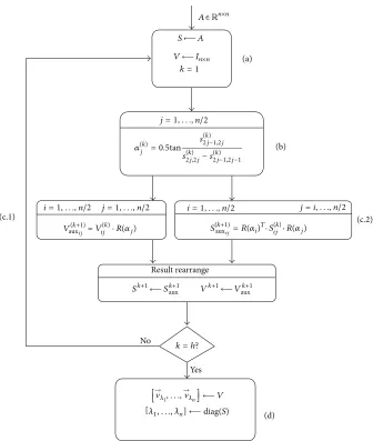
Figure1shows a functional diagram of the Jacobi algo-rithm. Since the C programming language was used, each task was implemented as aforloop and labeled to make optimization easier.

When the design starts its operation (a), the input matrix

𝐴 ∈R𝑛×𝑛is buffered in a memory element𝑆. In addition, to compute eigenvectors,𝑉(1)is loaded with an identity matrix (𝐼 ∈R𝑛×𝑛). After the initial operations, there are three tasks (a, b, and c) to be performedℎtimes in the external loop, whereℎcorresponds to the total number of Jacobi iterations (elimination of the𝑛elements adjacent to the main diagonal) that the algorithm will execute and is selected in such way that eigenvector error is minimized.

The first task that must be done in each Jacobi iteration (b) is to calculate rotation angles (𝛼_𝑗(𝑘)). As previously mentioned, this was achieved using the CORDIC algorithm in vectoring mode.

The next tasks to be performed (c.1 and c.2) are eigenvalue and eigenvector rotations, which consist of pre- and post-multiplication with the Givens rotation matrix. Since there are no data dependencies between these two tasks, they are placed in different loops and thus parallelization is possible. Pre- or postmultiplication with a Givens rotation matrix can be expressed as two vector rotations, so it can be performed with two rotation mode CORDIC algorithm executions. This leaves us with six CORDIC executions, four of them which correspond to eigenvalue calculation and the other two to eigenvector computation.

The final operation to be performed before the next Jacobi iteration (d) is a series of row and column permutations with the purpose of introducing new nonzero elements into the diagonal submatrices.

This element rearrangement was implemented as described by Brent and Luk [19] but with some modifications. In their study, they proposed a systolic architecture where each submatrix corresponded to an independent hardware unit called a processor, and all processors were interconnected so that data interchanges were possible.

Since our design did not have a defined hardware archi-tecture at this point, element interchange was substituted with the corresponding row and column permutations in order to fulfill the requirement of introducing new nonzero elements into the diagonal submatrices.

Finally, when all the Jacobi rotations are completed, eigenvalues and eigenvectors are output as arrays, which can be implemented as BRAM ports or AXI buses so that the design can be integrated in different kinds of system.

All tasks were implemented in the C programming language using a fixed point data type, following theXQN

quantification scheme, where a number is represented by𝑋 bits of integer part and𝑁bits of fractional part, with a total

number of bits (word length) of WL= 𝑋 + 𝑁 + 1for signed values and WL= 𝑋 + 𝑁for unsigned values.

Starting from the initial C prototype, different hardware architectures can be considered depending on the design requirements. Mainly, resource usage (LUT, Flip-Flops, mul-tipliers, memory elements) and timing performance (latency (𝑇_𝐿), throughput or initiation interval (II) and maximum clock frequency) are the parameters that we attempt to optimize:

(i) the latency (𝑇_𝐿), which specifies how much time will take until the system generate the first valid result; (ii) the initiation interval (II), which corresponds to the

throughput or the number of clock cycles between two valid sets of results, after the latency period.

As a result of the Vivado HLS optimization directives three architectures can be achieved, depending on which parameters are considered more important.

(i)Serial architecture: this hardware scheme pursues minimal resource usage at the expense of a higher latency. To reach this optimization level, a pipeline directive is specified on the external loop of the design, which performs the Jacobi iterations. (ii)Parallel architecture: in this kind of system, the main

goal is to achieve the best performance in terms of execution time (latency and throughput) at the expense of resource usage. To achieve this, pipeline is applied to the entire design, which means that the external loop will be unrolled and parallelism between two algorithm executions will be possible. (iii)Semiparallel architecture: although timing is still

important in this scheme, resource usage is also considered, and attempts are made to minimize it while affecting execution time as little as possible. In our particular case, this was achieved by limiting the number of CORDIC instances of the design in the parallel architecture.

Although all three alternatives were analyzed, the full parallel architecture was found to use a massive amount of internal FPGA resources, greatly exceeding the capacity of the device. This was mainly due to an excessive amount of CORDIC units in the rotation mode, which led to 55 hardware instances of it in the case of an 8 × 8 input matrix. Consequently, we ruled out the possibility of parallel architecture.

It is important to clarify the difference between semi-parallel and serial architecture. In both cases, we always attempted to maximize concurrency between operations, such as arithmetic operations and memory accesses; however, with parallel architecture it was also possible to achieve concurrence between two full executions of the algorithm.

(6)

S A

V In×n

k = 1

𝛼(k)_j = 0.5tan s

(k) 2j−1,2j

s(k)_2j,2j− s(k)_{2j−1,2j−1}

Sk+1 Sk+1aux Vk+1 Vauxk+1

(k+1)_{= V}(k)

ij · R(𝛼j)

i = 1,. . .,n/2 j = 1,. . .,n/2 _{i = 1},_{. . .},_n/2 j = i,_{. . .},_n/2

(k+1)_{= R(𝛼i}₎T_{· S}(k)

ij · R(𝛼j)

k = h?

(a)

(b)

(c.2)

(d) (c.1)

Result rearrange

No

[ ]

Yes

A∈Rn×n

Vaux𝑖𝑗 Saux𝑖𝑗

←− ←−

→

,_{. . .},→ _←−_V

𝜆1,. . .,𝜆n diag(S)

⌈⌉ ⌈⌉

←−

𝜆1 𝜆n

j = 1,_{. . .},n/2

Figure 1: Jacobi algorithm functional diagram.

semiparallel and serial architecture was limited to different values, allowing Vivado HLS to redesign the RTL implemen-tation and subsequently analyzing the design performance obtained.

First, we analyze the case of the semiparallel architecture. Since8 × 8is a common size in the literature for input matri-ces, the design was optimized for this matrix size, extending the conclusions reached to other matrix sizes. The results obtained (resource consumption and timing performance) are shown in Figure2.

An analysis of timing performance indicated that although latency did not vary very much, the initiation interval (II) was considerably reduced when the number of rotation mode CORDIC instances was increased from one to four, slowly decreasing as more CORDIC modules were added.

This result was mainly due to data dependencies between operations performed in the Jacobi algorithm. As previously

indicated, four rotations must be performed for eigenvalue calculation, and the result of the first two is required to perform the last two, whereas two independent rotations must be performed for eigenvector calculation.

From this, it can be concluded that four CORDIC modules will greatly increase the performance of the system. When timing performance is related to resource usage, it is clear that it increased linearly with CORDIC module usage, and the slope variation was due to the different control logic implemented by Vivado with an odd and an even number of CORDIC modules.

The last conclusion that can be reached from Figure2is that there was parallelism between two algorithm iterations, since𝑇_𝐿 > II. This means that the first valid result will be obtained after 𝑇_𝐿 clock cycles, but the next results will be obtained more rapidly, after every II clock cycles.

(7)

1 2 3 4 5 6 7 8 9 0

20 40 60 80 100

Dis

cr

et

e elemen

ts (%)

Resource usage

LUT FF

1 2 3 4 5 6 7 8 9

0 500 1000 1500 2000

Rotation CORDIC modules Rotation CORDIC modules

Execution time (clock cycles)

II TL

n·

TCLK

Figure 2: Semiparallel architecture implementation results of the Jacobi algorithm for8 × 8matrices.

was no parallelism between two algorithm executions and they only differed in one clock cycle that the system needed to start the next execution (II= 𝑇_𝐿+ 1).

As indicated earlier, the execution time between two valid result sets is the same as the latency period (𝑇_𝐿), and in the semiparallel design alternative, it evolved similarly to the initiation interval.

For similar reasons, there was a greater improvement in latency in the first four CORDIC module additions, which did not decrease at all after six. The increase in resource usage was also linear, now with a constant slope, although it used fewer resources.

4. Assessment of Design Parameters

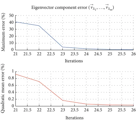
4.1. Optimal Number of Jacobi Iterations. To evaluate the quality of the results obtained using the Jacobi method, we conducted an experimental error analysis to determine how many Jacobi iterations were required to obtain satisfactory results.

The word length (WL) selected for the fixed point cod-ification scheme presented in Section2 was 18 bits with a fractional part of 15 bits (2Q15), since Xilinx FPGA multiplier entry is fixed to this value and the purpose of using the CORDIC algorithm was to minimize resource usage. In addition, as will now be shown, this codification provided sufficient precision to avoid overflow and growing rounding errors.

Simulating the system for multiple8 × 8real and sym-metric random matrices, we calculated the eigenvalue and

1 2 3 4 5 6 7 8 9

0 10 20 30 40 50

Dis

cr

et

e elemen

ts

Resource usage

1 2 3 4 5 6 7 8 9

1500 2000 2500 3000

Rotation CORDIC modules Rotation CORDIC modules

Execution time LUT

FF

TL

n·

TCLK

Figure 3: Serial architecture implementation results of the Jacobi algorithm for8 × 8matrices.

21 21.5 22 22.5 23 23.5 24 24.5 25 25.5 26

0 10 20 30 40 50

M

axim

um er

ro

r (%)

Iterations

21 21.5 22 22.5 23 23.5 24 24.5 25 25.5 26

0 0.2 0.4 0.6 0.8 1

Quadra

tic me

an

er

ro

r (%)

Iterations

Eigenvector component error (→_𝜆1,. . .,→_𝜆m)

Figure 4: Eigenvectors maximum and quadratic component error.

eigenvector maximum (𝑒MAX) and quadratic (𝑒SQRT) error,

comparing FPGA Jacobi fixed point results with MATLAB floating point implementation (eig).

(8)

the eigenvector component error, calculated according to the following expressions:

𝑒_%= 󵄨󵄨󵄨󵄨𝑉HLS󵄨󵄨󵄨󵄨 − 󵄨󵄨󵄨󵄨𝑉MATLAB󵄨󵄨󵄨󵄨

󵄨󵄨󵄨󵄨𝑉MATLAB󵄨󵄨󵄨󵄨 ⋅ 100,

𝑒MAX =max(󵄨󵄨󵄨󵄨𝑒%󵄨󵄨󵄨󵄨),

𝑒SQRT =

1

𝑘2√

𝑘−1

∑

𝑖=0

𝑒2

%,

(20)

where𝑘represents the total number of samples. The error obtained was plotted as a function of the number of Jacobi iterations (i.e., the number of rotations performed for each submatrix) and was used to determine the optimal number of iterations (ℎ) that the algorithm must perform to obtain sufficiently accurate results.

Our analysis of 8 × 8 matrices indicated that ℎ = 26 was the best number of iterations for both eigenvectors and eigenvalues in order to obtain a sufficiently accurate solution, since the error was constant from this value on.

After performing the same tests for other input matrix sizes, it was concluded that, in general, expression(21)can be used to determine the optimal number of iterations to be performed for an𝑛 × 𝑛matrix:

ℎ = 9 + 𝑛log𝑛. (21)

4.2. Serial/Parallel Jacobi Analysis. Since an expression was available for the optimal number of Jacobi iterations (ℎ), we also conducted a study of the design performance depending on initial matrix size.

With the parallel architecture, we found that although the Vivado HLS generated an RTL design for matrices with an order 𝑛 > 10, the Vivado suite synthesizer was unable to implement it successfully. However, the serial architecture design performed well for higher order matrices (20 × 20).

Based on the parametric study performed in Section3, we decided that a good trade-off between execution time and resource usage would be to use four CORDIC modules, which would perform WL− 1iterations in both parallel and serial architectures, where WL was the data word length.

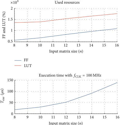
Implementation results for the serial architecture are shown in Figure5for the Xilinx Artix 7 series (XC7A100T-1CSG324C) device.

Turning first to resource usage, it can be seen that this did not not increase as fast as execution time, since when matrix size is increased with a fixed amount of CORDIC units, only storage elements and control logic will be added. Consequently, it becomes evident that in terms of resources used, the design has an𝑂(𝑛2)complexity.

Regarding execution time (𝑇exe), the Vivado HLS enabled

us to examine the sequence of operations performed by the design in each clock cycle. An analysis of this information indicated that the design latency, which corresponds to execution time in the serial architecture, follows the following expression:

𝑇_𝐿= 𝑇load+ 𝑛2⋅ ℎ, (22)

8 9 10 11 12 13 14 15 16

0.5 1 1.5 2

Used resources

FF a

n

d L

UT (%)

8 9 10 11 12 13 14 15 16

0 50 100 150

FF LUT

Input matrix size (_n)

Input matrix size (n)

Execution time with 100MHz

×104

Texe

(

𝜇

s)

fCLK=

Figure 5: Serial Jacobi design performance with matrix order increase.

where 𝑛 is the size of the processed matrix and ℎ is the number of Jacobi iterations performed, following expression

(21). Meanwhile,𝑇load (23)corresponds to the time required

to read sufficient data from an external memory to start the first Jacobi iteration, and𝑛2 is the amount of clock cycles required to perform a Jacobi iteration:

𝑇load=

𝑛2

2 +

𝑛

2+ 4. (23)

A similar study was performed for different numbers of rotation CORDIC units, which revealed that the time to perform a Jacobi iteration varied. However, it remained a function of𝑛2, so system latency (𝑇_𝐿) was still related to the size of the input matrix, as shown in the following expression:

𝑇_𝐿= 𝑇load+ 𝑇𝐽⋅ ℎ, (24)

where𝑇_𝐽 = 𝑓(𝑛2)is the time required to perform a Jacobi iteration.

(9)

Design comparison

11000 23000 34000 45000 LUT

8500 17000 26000 34000

FF

4000 8000 12000 16000

4000

8000

12000

16000

Semiparallel Jacobi Serial Jacobi Floating point QR MUSIC (Xu et al., 2008) VHDL (Bravo et al., 2008) Vivado HLS library

TL(nTCLK)

II(

nTCLK

)

Figure 6: Comparative between different design alternatives.

5. Comparison with Other Proposals

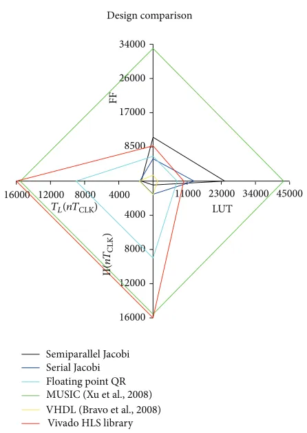
The results obtained were also compared with those reported in other studies of8 × 8matrices, since these have received much research attention.

Figure6 shows the implementation results for the two architectures proposed here (serial and parallel), a Jacobi serial architecture carried out in VHDL [1], a Jacobi semi-parallel architecture from the multiple signal classification (MUSIC) algorithm [8], and the Vivado HLS linear algebra library svd implementation.

The criteria selected to compare the different designs were as follows: FPGA resource consumption, in terms of the discrete elements FF and LUT, computation time (latency and initiation interval), and maximum clock frequency (𝑓CLK).

The VHDL serial Jacobi algorithm features a fully cus-tomized system using two ad hoc CORDIC modules, one of which works in rotation and vectoring mode while the other is optimized to work only in rotation mode.

The Jacobi module used in the MUSIC algorithm features a semiparallel architecture based on the Brent and Luk proposal [12] and also uses the CORDIC algorithm for the calculations. However, it does not implement the full systolic array, only making use of a subset of this to save resources.

Turning first to the two Jacobi algorithm implementations proposed here, it is evident that the best performance in terms of speed was achieved by the semiparallel architecture, whereas the serial architecture only used half of the resources required to implement the parallel one.

Vivado HLS library

Clock frequency (MHz) VHDL

(Bravo et al., 2008)

QR

Parallel Jacobi

Serial Jacobi

0 50 100 150 200 250 300

Figure 7: Maximum clock frequency for all the designs when input matrix size is fixed to8 × 8.

The other Vivado HLS implementation considered was the svd function from the Vivado HLS library, which can only be implemented in single precision floating point for-mat. Resource usage is not dissimilar to our Vivado HLS implementations; however, it is slower and makes use of 58 DSP48E blocks.

The difference arises from the use of floating point cores which are implemented with DSP units, while the fixed point CORDIC approach employed in the present study only required two DSP48E multipliers per unit.

As previously mentioned, a floating point QR algorithm was implemented in the same FPGA device also using Vivado HLS. The main purpose of this was to determine whether other algorithms presented greater computational efficiency than the Jacobi method. Although we used different coding systems in the Jacobi and QR algorithms, respectively, an analysis of both implementations revealed that QR was less suitable for a hardware implementation since the operations performed can vary between different iterations.

Nevertheless, we found that although the performance of the algorithm in terms of execution time was poor, it did not use a large amount of FPGA resources, and it therefore represents an alternative to consider when floating point codification is required.

Looking next at the eigen solver implemented as part of the MUSIC algorithm, it can be seen that it did not perform very well. On paper, it is similar to the semiparallel architec-ture presented here, but the control logic was designed by hand. This shows that HLS performs better than traditional hardware design flows when control logic becomes too complicated, since it is implemented automatically.

Our final comparison was with the VHDL serial architec-ture, in which only two CORDIC modules were used. Since everything in this design was customized for the application, timing performance was similar to HLS designs, but it used far fewer resources.

As regards the maximum clock frequency at which the designs can work, Figure7 shows a comparison of all the alternatives discussed.

(10)

On the other hand, we find the VHDL design. In this case, the performance of the design proposed in [1] was similar to the floating point designs since it was hand-coded at a very low optimization level.

6. Conclusions

In this paper, we have described a high level synthesis implementation of the Jacobi algorithm for eigenvalue and eigenvector calculations, and this has been compared to similar or related systems reported in the literature.

The main purpose of using a HLS tool was to try to achieve a similar performance to that of a custom RTL system coded in, for example, VHDL, in a fraction of the design time required.

In recent years, the amount of resources available in FPGA devices has grown exponentially, and thus rapidity is becoming more important than efficiency when implement-ing computational algorithms.

Furthermore, HLS tools have evolved, making it possible to achieve good systems that are easy to integrate into larger designs as hardware coprocessors together with a CPU, or as a processing block in regular RTL designs.

As final paper conclusion, we can say that the use of high level implementation tools reduce the design time. In most cases, the designs are initially coded, simulated, and validated with high level languages, where there exist standard libraries and reference code available. Manual RTL coding is not usually an easy step because there is not a straight way to translate the functional algorithm to RTL description. In addition, the required level of RTL expertise is very high.

Another inconvenience for RTL-based designs appears when new changes have to be included in the algorithm. The RTL structure is not very flexible and any modification to the algorithm requires a lot of time (simulation and recoding). Nevertheless, RTL designs generate hardware reconfigurable approaches with less resources and higher clock frequency than high level hardware designs (see Figures6and7).

The developed algorithm in this work was initially made with a traditional RTL flow [1]. As a result, we can compare the results of a complex algorithm such as Jacobi based on RTL or HLS flows. According to Figures6and7, the achieved results for the HLS methodology compared with RTL-based design are favorably from different points of view.

We have shown that the design process varies from the traditional RTL flow, since it is possible to iterate on the same code to obtain different hardware architectures and perform parametric simulations of the hardware in order to obtain the best results.

Therefore, the designer should balance what are the prior requirements in the system, clock frequency/resources, or design time and choose the methodology (RTL/HLS) that best fit for that particular case.

Conflict of Interests

The authors declare that there is no conflict of interests regarding the publication of this paper.

Acknowledgment

This work has been supported by the Spanish Ministry of Economy and Competitiveness through the ALCOR Project (DPI2013-47347-C2-1-R).

References

[1] I. Bravo, M. Mazo, J. L. Lázaro, P. Jiménez, A. Gardel, and M. Marrón, “Novel HW architecture based on FPGAs oriented to solve the eigen problem,”IEEE Transactions on Very Large Scale Integration (VLSI) Systems, vol. 16, no. 12, pp. 1722–1725, 2008. [2] H. Gao and R. Ma, “On a system modelling a population with

two age groups,”Abstract and Applied Analysis, vol. 2014, Article ID 920348, 5 pages, 2014.

[3] X. Tang, W. Deng, and Z. Qi, “Investigation of the dynamic stability of microgrid,”IEEE Transactions on Power Systems, vol. 29, no. 2, pp. 698–706, 2014.

[4] S. Wu, J. Zhang, Y. Hou, and X. Bai, “Convergence of gossip algorithms for consensus in wireless sensor networks with intermittent links and mobile nodes,”Mathematical Problems in Engineering, vol. 2014, Article ID 836584, 18 pages, 2014. [5] J. A. Jim´enez, M. Mazo, J. Ure˜na et al., “Using PCA in

time-of-flight vectors for reflector recognition and 3-D localization,”

IEEE Transactions on Robotics, vol. 21, no. 5, pp. 909–924, 2005. [6] W. Haiqing, S. Zhihuan, and L. Ping, “Improved PCA with optimized sensor locations for process monitoring and fault diagnosis,” inProceedings of the 39th IEEE Confernce on Decision and Control, vol. 5, pp. 4353–4358, December 2000.

[7] A. A. S. Ali, A. Amira, F. Bensaali, and M. Benammar, “PCA IP-core for gas applications on the heterogenous zynq platform,” inProceedings of the 25th International Conference on Microelec-tronics (ICM ’13), pp. 1–4, December 2013.

[8] D. Xu, Z. Liu, X. Qi, Y. Xu, and Y. Zeng, “A FPGA-based implementation of MUSIC for centrosymmetric circular array,” in Proceedings of the 9th International Conference on Signal Processing (ICSP ’08), pp. 490–493, October 2008.

[9] J. H. Wilkinson,The Algebraic Eigenvalue Problem, Monographs on Numerical Analysis, Clarendon Press, New York, NY, USA, 1988.

[10] S. Sundar and B. K. Bhagavan, “Generalized eigenvalue prob-lems: Lanczos algorithm with a recursive partitioning method,”

Computers & Mathematics with Applications, vol. 39, no. 7-8, pp. 211–224, 2000.

[11] D. P. O’Leary and P. Whitman, “Parallel QR factorization by householder and modified Gram-Schmidt algorithms,”Parallel Computing, vol. 16, no. 1, pp. 99–112, 1990.

[12] R. P. Brent, F. T. Luk, and C. van Loan, “Computation of the generalized singular value decomposition using mesh-connected processors,”Journal of VLSI and Computer Systems, vol. 1, no. 3, pp. 242–270, 1983.

[13] J. E. Volder, “The CORDIC trigonometric computing tech-nique,”IRE Transactions on Electronic Computers, vol. EC-8, no. 3, pp. 330–334, 1959.

[14] J. R. Cavallaro and F. T. Luk, “CORDIC arithmetic for an SVD processor,”Journal of Parallel and Distributed Computing, vol. 5, no. 3, pp. 271–290, 1988.

(11)

[16] Impulse C,http://www.impulseaccelerated.com/tools.html. [17] Catapult c,http://calypto.com/en/products/catapult/overview/. [18] Vivadohlsxilinx web page, http://www.xilinx.com/products/

designtools/vivado/integration/esl-design.htm.

[19] R. P. Brent and F. T. Luk, “The solution of singular-value and symmetric eigenvalue problems on multiprocessor arrays,”

Society for Industrial and Applied Mathematics, vol. 6, no. 1, pp. 69–84, 1985.

[20] C.-C. Sun, J. G¨otze, and G. E. Jan, “Parallel Jacobi EVD methods on integrated circuits,”VLSI Design, vol. 2014, Article ID 596103, 9 pages, 2014.

[21] Y. Liu, C.-S. Bouganis, and P. Y. K. Cheung, “Hardware architec-tures for eigenvalue computation of real symmetric matrices,”

IET Computers and Digital Techniques, vol. 3, no. 1, pp. 72–84, 2009.

[22] W. Ford, Numerical Linear Algebra with Applications: Using MATLAB, Academic Press, New York, NY, USA, 1st edition, 2014.

[23] S. W. Kang and S. N. Atluri, “Application of nondimensional dynamic influence function method for eigenmode analysis of two-dimensional acoustic cavities,”Advances in Mechanical Engineering, vol. 2014, Article ID 363570, 9 pages, 2014. [24] Á. Bernal, R. Miró, D. Ginestar, and G. Verdú, “Resolution of

the generalized eigenvalue problem in the neutron diffusion equation discretized by the finite volume method,”Abstract and Applied Analysis, vol. 2014, Article ID 913043, 15 pages, 2014. [25] W. Gafsi, F. Najar, S. Choura, and S. El-Borgi, “Confinement of

vibrations in variable-geometry nonlinear flexible beam,”Shock and Vibration, vol. 2014, Article ID 687340, 7 pages, 2014. [26] G. H. Golub and C. F. Van Loan,Matrix Computations, Johns

Hopkins Studies in the Mathematical Sciences, Johns Hopkins University Press, Baltimore, Md, USA, 4th edition, 2013. [27] J. S. Walther, A Unified Algorithm for Elementary Functions,

1972.

[28] B. Lakshmi and A. S. Dhar, “CORDIC architectures: a survey,”

VLSI Design, vol. 2010, Article ID 794891, 19 pages, 2010. [29] J. Faires and R. L. Burden,Numerical Methods, Brooks Cole

(12)

Submit your manuscripts at

http://www.hindawi.com

Hindawi Publishing Corporation

http://www.hindawi.com Volume 2014

Mathematics

Journal of

Mathematical Problems in Engineering

Hindawi Publishing Corporation http://www.hindawi.com

Differential Equations

International Journal of

Volume 2014

http://www.hindawi.com Volume 2014 Hindawi Publishing Corporationhttp://www.hindawi.com Volume 2014

http://www.hindawi.com Volume 2014 Mathematical PhysicsAdvances in

Complex Analysis

Journal of

Optimization

Journal of

Combinatorics

International Journal of

Journal of

Function Spaces

Abstract and Applied Analysis

International Journal of Mathematics and Mathematical Sciences

Hindawi Publishing Corporation http://www.hindawi.com Volume 2014

The Scientific

World Journal

Discrete Dynamics in Nature and Society Hindawi Publishing Corporation

Discrete Mathematics

Journal of

http://www.hindawi.com Volume 2014 Hindawi Publishing Corporationhttp://www.hindawi.com Volume 2014