NEW HEURISTICS FOR THE NO-WAIT FLOWSHOP WITH SEQUENCE-DEPENDENT SETUP
TIMES PROBLEM
Daniella Castro Araújoa; Marcelo Seido Naganoa
a University of São Paulo (USP), São Paulo, SP, Brazil
ABEPRO
DOI: 10.14488/BJOPM.2015.v12.n2.a1
In this paper, we address the problem of scheduling jobs in a no-wait flow shop with sequence-dependent setup times with the objective of minimizing the make span and the total flow time. As this problem is well-known for being NP-hard, we present two new constructive heuristics in order to obtain good approximate solutions for the problem in a short CPU time, named GAPH and QUARTS. GAPH is based on a structural property for minimizing make span and QUARTS breaks the problem in quartets in order to minimize the total flow time. Experimental results demonstrate the superiority of the proposed approaches over three of the best-know methods in the literature: BAH and BIH, from Bianco, Dell´Olmo and Giordani (1999) and TRIPS, by Brown, McGarvey and Ventura (2004).
Keywords: Heuristic, No-wait Flow shop, Sequence-Dependent Setup, Make span, Total flow time. Abstract
INTRODUCTION
The first systematic approach to scheduling problems was undertaken in the mid-1950s. Since then, thousands of papers on different scheduling problems have appeared in the literature. The majority of these papers assumed that the setup time is negligible or part of the job processing time. Treating setup times separately from processing times allows operations to be performed simultaneously and hence improves resource utilization. This is, in particular, important in modern production management systems such as just-in-time (JIT), optimized production technology (OPT), group technology (GT), cellular manufacturing (CM), and time-based competition (ALLAHVERDI et al., 2008).
Another important area in scheduling arises in no-wait flow shop problems (NWFSP), where jobs have to be processed without interruption between consecutive machines. There are several industries where the no-wait flow shop problem applies including the metal, plastic, and chemical industries. As noted by Hall and Sriskandarajah (1996), the first of two main reasons for the occurrence of a no-wait or blocking production environment lies in the production technology itself. In some processes, for example, the temperature
or other characteristics (such as viscosity) of the material require that each operation follow the previous one immediately. According to Bianco .et al., (1999), flow shop no-wait scheduling problems are also motivated by concepts such as JIT and zero inventory in modern manufacturing systems.
A survey on NWFSP has been conducted by Hall and Sriskandarajah (1996), where several practical applications
are shown. Allahverdi.et al., (1999, 2008) provided a
comprehensive review of the literature on scheduling
problems with setup times. The NWFSP with sequence dependent setup times with the objective of minimizing make span was first proposed by Bianco et al.,(1999). They showed how to reduce this problem to the asymmetric travelling salesman problem (ATSP) and presented two lower bounds and two heuristics, named BAH and BIH. The computational results showed that BIH outperformed BAH in the solutions quality. Kumar et al.,(2000) considered a
NWFSP that used lot-streaming to improve productivity. They developed a TSP formulation for the multi-product and continuous-sized case and proposed a heuristic to obtain an optimal sequence for integer-sized sublots.
for the problem, where the setup and
processing times satisfy certain conditions, and presented five heuristics for the general problem. Later, Allahverdi
et Aldowaisan (2001) considered the
problem and presented five heuristics that used a repeated insertion technique. Stafford et Tseng (2002) proposed two mixed-integer linear programming (MILP) models to solve
the m-machine NWFSP with sequence dependent setup times in order to minimize the make span. Aldowaisan
et Allahverdi (2003) proposed six heuristics based on simulated annealing and genetic algorithms techniques
for the problem. The simulated annealing
based heuristics performed better than the others. Fink
et Voβ (2003) proposed three constructive heuristics and several meta-heuristics for the NWFSP with total flowtime as the criteria. Shyu et al., (2004) presented an ant colony
optimization algorithm for the problem, and showed that their algorithm outperformed earlier
heuristics.. Brown et al., (2004) presented a non-polynomial time solution method and a heuristic named TRIPS for the NWFSP with sequence independent setup times, considering for the performance measures both the total flow time
and make spanRuiz et al.,(2005) addressed the
problem and proposed two genetic algorithms, named GA and HGA.. França et al., (2006) considered the same problem
as. Bianco et al., (1999) and solved it by an evolutionary approach. Their genetic algorithm outperformed BIH. Ruiz
et Allahverdi (2007a) presented a domination relation for
the problem and proposed an iterated
local search method and five heuristics for the same
problem with m-machines. The results showed that three of their heuristics outperformed TRIPS and the ant colony algorithm of Shyu et al., (2004). Ruiz et Allahverdi (2007b)
proposed seven heuristics and four genetic algorithms for the NWFSP with sequence independent setup times in order to minimize the maximum lateness. Their genetic algorithms outperformed the heuristics of Ruiz et Allahverdi (2007a).
Grabowski et Pempera (2007) developed and compared
five heuristcs for the problem. In order to
decrease the computational effort, they used multimoves.
Ruiz et Stüzle (2008) presented two simple local search
based iterated greedy algorithms for both and
problems, and showed that their algorithms
performed better than GA and HGA. Framinan et Nagano
(2008) studied the problem and proposed
a heuristic based on an analogy between the problem under consideration and the travelling salesman problem (TSP). Pan et al., (2008) presented a discrete particle swarm optimization (DPSO) to solve the NWFSP with both make span and total flow timecriteria. The results showed that the algorithm outperformed the heuristics of Grabowski
et Pempera (2007) and Fink et Voβ (2003). Yaurima et al.,(2009) proposed a genetic algorithm for the hybrid flow shop problem with unrelated machines, sequence dependent setup times, availability constraints and limited buffer, and introduced a crossover operator and stopping criterion to improve the solution quality. Eren (2010) proposed an integer programming model to solve the flow shop problem with sequence dependent setup times. The objective function was the weighted sum of total completion time and the make span. The model could solve problems up to six machines and eighteen jobs. Wang (2010) considered the NWFSP with maximum lateness criterion and developed properties to reduce the time to evaluate a candidate in a tabu search approach. Framinan et al., (2010) addressed the
problem and proposed a constructive heuristic based on an analogy with the two-machine problem. The computational results showed that the heuristic outperformed existing ones regarding the solution quality.
In this paper, we consider the problem of scheduling
a no-wait flow shop problem with sequence dependent
setup times ( ), which consists of a set of n jobs which are to be processed on a
set of m dedicated machines,
each one being able to process only one job at a time.
Job consists of m operations ,
to be executed in this order, where operation must
be executed on machine k, with processing time, immediately before operation . There is a sequence dependent setup time between operations and
the time break between the beginning of job and the beginning of job at machine k, where, is the job of
occupying position i in σ. QUARTS breaks the problem in quartets, reducing the required computational effort to find the solution.
EXISTING CONSTRUCTIVE HEURISTICS FOR THE PROBLEM
In this section, we review the main contributions to the problem regarding constructive methods. More specifically, we explain in detail the constructive heuristics BAH and BIH, from Bianco et al., (1999) and TRIPS, from Brown et al.,(2004). BAH and BIH were made for the no-wait flow shopwith sequence-dependent setup times in order to minimize the make span, and were adapted in this work to also minimize the total flow time. TRIPS was made for the no-wait flow shop with sequence-independent setup times, to minimize both the make span and total flow time , and was adapted in this work to the no-wait flow shopwith sequence-dependent setup times.
BAH
BAH algorithm finds a feasible sequence in n iterations. At each iteration, given a partial sequence of the scheduled jobs computed in the previous iteration, the algorithm examines a set of candidates of the unscheduled jobs, and appends a candidate job to a partial sequence minimizing the time when the shop is ready to process an unscheduled
job.
The pseudo-code of the heuristic is as follows:
Given a set of n jobs, let σ be the set
of programmed jobs and U be the set of non-programmed jobs.
Step 1: ; ;
Step 2: While , do:
Step 2.1: Choose the job to be added at the end
of the sequence , such that the makespan/flowtime is
minimum;
Step 2.2: Add job to the end of the sequence σ;
Step 2.3: .
BIH
The BIH algorithm also finds a sequence of n jobs on n
iterations. But in this algorithm, at each iteration it considers
a sequence of a subset of jobs, and finds the best sequence obtained inserting an unscheduled job in any position of the given sequence.
A more detailed description of the heuristic is as follows: Given a set of n jobs, let σ be the
set of programmed jobs, U be the set of non-programmed jobs and h the relative insertion position.
Step 1: ; ;
Step 2: While , do:
Step 2.1: Choose the job which can be inserted
in the sequence , such that the make span/flow time is minimum. Let h bethe relative insertion position;
Step 2.2: Insert job at position h in the sequence σ;
Step 2.3: .
TRIPS
TRIPS examines all possible three-job combinations from
the set of unscheduled jobs and chooses the sequence that minimizes the three-job objective. Then,
assigns job to the last empty position in the sequence σ and removes from U. The heuristic repeats the process, assigning one more job to σ for each set of triplets examined until only three jobs are left. Then, it selects the optimal sequence for these jobs and places them in the final positions of heuristic sequence σ.
The pseudo-code of the heuristic is as follows:
Given a set of n jobs, let σ be the set
of programmed jobs and U be the set of non-programmed jobs.
Step 1: ; ; h ;
Step 2: While h<n-2, do:
Step 2.1: Given that the first h jobs are assigned in
sequence , compare all ordered triplets of jobs from ;
Step 2.2: Choose the triplet such that the
make span/flow time is minimized for jobs in
positions h+1, h+2, h+3, respectively, of sequence .
Step 2.3: Place in position h+1 of ;
Step 2.4: h h+1; ;
A STRUCTURAL PROPERTY FOR THE NEW HEURISTIC FOR MAKESPAN
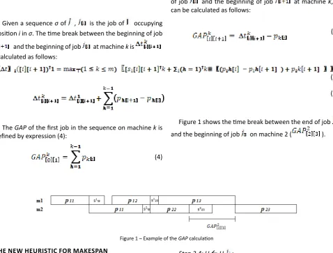
Given a sequence σ of , is the job of occupying position i in σ. The time break between the beginning of job
and the beginning of job at machine k is , calculated as follows:
Defining as the time break between the end
of job and the beginning of job at machine k, it can be calculated as follows:
(1)
(2)
(3)
The GAP of the first job in the sequence on machine k is
defined by expression (4):
(4)
Figure 1 shows the time break between the end of job
and the beginning of job on machine 2 ( ).
Figure 1 – Example of the GAP calculation THE NEW HEURISTIC FOR MAKESPAN
The new heuristic proposed in this paper will be called GAPH – Gap Heuristic. The pseudo-code of the algorithm is given next:
Given a set of n jobs, let U be the set of non-programmed jobs and
be the sequence of n jobs scheduled, where x = {1,2,3,4}. Calculate the of each job i = 1, ..., n to each job j
= 1, ..., n at all m machines.
Step 1:UJ; Ø;
Step 2: While U ≠ Ø, do:
Step 2.1: Calculate the total cost* on the last machine for
all possible insertions of each job in the sequence . Let h be the relative insertion position;
Step 2.2: Choose the job that gives the lower total cost
at position h;
Step 2.3: Insert job at position h of the sequence ;
Step 2.4:UU- ;
Step 3:UJ; Ø
Step 4: While U ≠ Ø, do:
Step 4.1: Calculate the total GAP** for all possible
insertions of each job in the sequence . Let h be
the relative insertion position;
Step 4.2: Choose the job that gives the lower total GAP
at position h;
Step 4.3: Insert job at position h of the sequence ;
Step 4.4:UU- ;
Step 5:UJ; Ø;
Step 6: While U ≠ Ø, do:
Step 6.1: Calculate the sum of the GAPs on the last
machine for all possible insertions of each job in
the sequence . Let h be the relative insertion position;
Step 6.2: Choose the job that gives the lower sum of (3)
The sum of the GAPs with the processing time
of the job to be inserted on the last machine is:
.
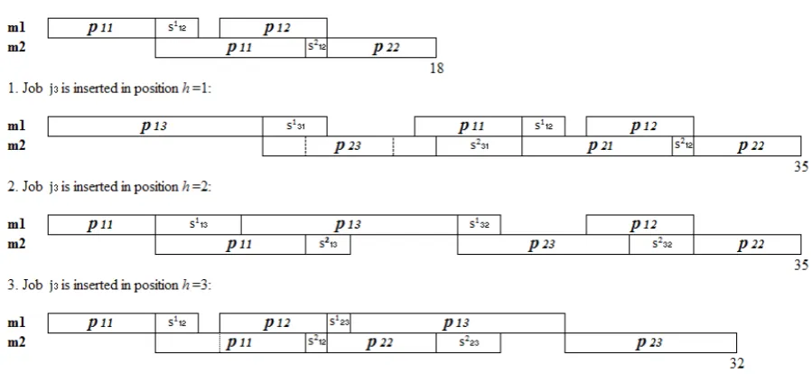
Figure 4 shows how the method works for each pair of steps (1-2; 3-4; 5-6; 7-8). In the example, jobs and were
already scheduled ( ) and job is scheduled on each possible position of the sequence (h).
the GAPs on the last machine at position h;
Step 6.3: Insert job at position h of the sequence ;
Step 6.4:UU- ;
Step 7:UJ; Ø;
Step 8: While U ≠ Ø, do:
Step 8.1: Calculate, for all possible insertions of each job in the sequence , the sum of the GAPs with the
processing time of the job on the last machine. Let h be the
relative insertion position;
Step 8.2: Choose the job that gives the lower sum of the GAPs with the processing time of the job on the
last machineat position h;
Step 8.3: Insert job at position h of the sequence .
Step 8.4:UU- ;
Step 9: Choose, among the sequences , the one with the lower make span.
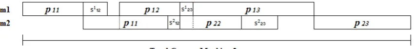
*The total cost on a k machine is defined as the scheduling total time on this machine. Thus, the total cost encompasses the sum of the GAPs on machine k with the scheduled
operations processing times on that machine. Note that the
total cost on the last machine is equivalent to the (see Figure
2).
Figure 2 – Example of the total cost
**The total GAP is the sum of all GAPs in all machines.
In Figure 3, the total GAP is:
The sum of the GAPs on the last machine is: .
Figure 4 – Numerical example of how the method works
For example, if the method were on the second step, the sequence chosen would be the third one, that gives the
lower total cost on the last machine.
DESCRIPTION OF THE NEW HEURISTIC FOR THE TOTAL FLOWTIME
Brown et al., (2004) presented the TRIPS heuristic detailed above. TRIPS breaks the problem in triplets, reducing the required computational effort to find the solution. We made some modifications in this heuristic in order to improve its results. The main difference of the proposed heuristic is that it breaks the problem in quartets, instead of triplets. The new heuristic will be called QUARTS.
In order to choose the two first jobs, QUARTS examines all possible four-job combinations from the set of jobs J
and chooses the sequence that minimizes the total flow time. Then assigns jobs and to the first and second positions of σ, respectively, and removes them from the set of non-scheduled jobs. In the next iteration, the job scheduled in the second position of σ will be the first position ( of all possible four-job combinations . The job in the second position ( )of the
quartet with the lowest flow time is then scheduled in the
next empty position of σ and is removed from the set of
non-scheduled jobs. Repeating this process, QUARTS assigns
one job in at each iteration, and the job scheduled in the previous iteration is always the first one of the quartets of the current iterations, until only three jobs are left. Select the optimal sequence for these jobs and place them in the final positions of heuristic sequence σ. Then, QUARTS tries to improve the solution found through a neighborhood insertion and a neighborhood permutation search
procedures, described as follows:
• Neighborhood Insertion Search:
Insert each job in the sequence σ at the (n-1)²
possible positions, being n the number of jobs. Choose
the insertion that obtains the lower total flowtime. • Neighborhood Permutation Search:
This search exchanges pairs of tasks in the sequence
, at the possible positions. Choose the insertion that obtains the lower total flowtime.
The pseudo-code of the algorithm is given next:
Given a set of n jobs, let U be the
set of non-programmed jobs and be
Step 1:UJ; ; h .
Step 2:
Step 2.1: Calculate the total flow time for all possible
four-job combination of U;
Step 2.2: Choose the quartet that gives the lower flow time and assign and in positions 1 and
2 of σ, respectively;
Step 2.3:h h+2; ; .
Step 3:While h<n-2, do:
Step 3.1: ;
Step 3.2: Calculate the flow time for all quartets
of U;
Step 3.3: Choose the quartet that gives the lower flow time and assign to the position h of σ;
Step 3.4:h h+1; ;
Step 4: Assign to the last positions, respectively, of σ. Calculate the total flow time.
Step 4.1: Calculate the total GAP** for all possible
insertions of each job in the sequence . Let h be
the relative insertion position;
Step 4.2: Choose the job that gives the lower total GAP
at position h;
Step 4.3: Insert job at position h of the sequence ;
Step 4.4:UU- ;
Step 5: Neighborhood insertion search: Considering all insertion neighborhood of sequence σ, determine the sequence that gives the lower total flow time. If the total
flow time of the sequence is lower than the sequence σ, then σ .
Step 6: Neighborhood permutation search: Considering all insertion neighborhood of sequence σ, determine the sequence that gives the lower total flow time. If the total flow time of the sequence is lower than the
sequence σ, then σ .
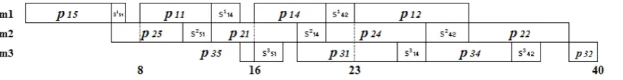
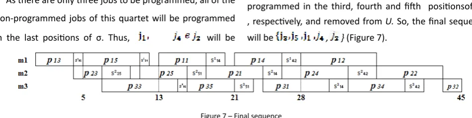
Figures 5, 6 and 7 give an example of the method, in a
problem with 5 jobs and 3 machines.
First of all, QUARTS calculates the flow time of all quartets . Then, it picks up the one with the lowest flow time. Figure 5 shows the selected quartet ( ).
Figure 5 – First selected quartet
The first and second jobs of the quartet
are then programmed in the first and second positions of the set of programmed jobs (σ), and are removed from the
set of non-programmed jobs (U). In the next iteration, job
will be the first position of all quartets.
After calculating the flow time of all quartets
, QUARTS picks up the one with the lowest flow time. Figure 6 shows the selected quartet ( ).
As there are only three jobs to be programmed, all of the non-programmed jobs of this quartet will be programmed in the last positions of σ. Thus, will be
programmed in the third, fourth and fifth positionsof , respectively, and removed from U. So, the final sequence
will be , } (Figure 7).
Figure 7 – Final sequence
Then, the heuristic tries to improve the result with the neighborhood insertion and permutation searches.
COMPUTATIONAL EXPERIENCE
The computational experience was carried out in two parts. In part I, we tested GAPH, BIH, BAH and TRIPS with the make span criteria. In part II, we tested QUARTS, BIH, BAH and TRIPS with the total flow time criteria. As stated, TRIPS heuristic was adapted to the no-wait flow time with sequence-dependent setup times problem, and BAH and BIH were adapted in order to also minimize the total flow time.
The heuristics were tested in the well-known tested of Taillard (1993). This tested contains twelve sets for a given combination of jobs and machines, i.e., n {20,50,100,200,500} and m {5,10,20}. We performed four experiments, one for
each of the four different sequence-dependent
Taillard-based instance sets from. (Ruiz et al. ,(2005). The tests
contain four different processing times to sequence-dependent setup times ratios. For example, the instance set SSD-10 is composed of one hundred twenty instances where the processing times are those of Taillard’s benchmark and where the sequence-dependent setup times are 10% of the processing times. In the instance set SSD-50, the setup times are 50% of the processing times and the instance sets SSD-100 and SSD-125 have setup times that are SSD-100% and 125% of the processing times respectively. So for example, if the processing times in Taillard’s instances are generated from a uniform distribution in the range [1; 99], in the SSD-10 instance set the setup times are uniformly distributed in the range [1; 9] ([1; 49], [1; 99] and [1; 124] for the instance sets SSD-50, SSD-100 and SSD-125 respectively). Thus, we have
four problem sets and a total of 480 different instances. The five hundred job instance was rather large and we chose to solve only the first one hundred ten instances (up to two hundred jobs and twenty machines).
The instances in the tested have been solved by the selected heuristics (coded in Python). Part I was solved in a computer with a Pentium IV 3.00GHz processor and 512MB
RAM, and Part II in a computer with a Intel Core 2 Duo
2.20GHz/2.20GHz processor and 4.00GBRAM.
Tables 1 and 2 summarize the result obtained for the make span criteria and Tables three and four for the total
flow time criteria in terms of the success percentage, the average relative percentage deviation (ARPD), and the average CPU time.
The success rate is defined by the ratio between the number of problems for which a particular method was the best solution and the total number of problems solved. Therefore, when two methods get the best solution for
the same problem, their percentages of success are both improved.
The ARPD consists of averaging the RPD over a number of
instances with the same number of jobs. We have grouped
the results for a given number of jobs and different machines, as the number of machines had almost no influence in the results. For a given objective function , the RPD obtained
by a heuristic H on a given instance is computed as follows:
(5)
where:
is the makespan/total flowtime computed by
method h;
is the best makespan/total flowtime computed by the methods.
Table 1 – Comparison of results in Taillard´s testbed SSD-10 and SSD-50 (Makespan)
SSD-10 SSD-50
n x m BAH BIH TRIPS GAPH BAH BIH TRIPS GAPH
20x5
0.00* 60 0 100 0 60 0 100
15.54** 1.83 9.27 0 13.13 1.27 7.23 0
0.03*** 0.11 0.34 0.27 0.03 0.11 0.34 0.27
20x10
0 50 0 100 0 70 0 100
15.87 2.48 8.23 0 14.21 1.59 8.09 0
0.06 0.15 0.37 0.31 0.06 0.15 0.36 0.31
20x20
0 60 0 100 0 70 0 100
13.42 0.42 8.82 0 13.21 0.88 8.37 0
0.18 0.26 0.43 0.43 0.17 0.26 0.42 0.43
Average
0 56.67 0 100 0 66.67 0 100
14.94 1.58 8.77 0 13.51 1.25 7.9 0
0.09 0.17 0.38 0.34 0.09 0.17 0.37 0.34
50x5
0 70 0 100 0 50 0 100
11.74 0.41 5.77 0 9.8 0.98 5.44 0
0.17 2.87 14.3 7.92 0.16 2.89 14.11 7.96
50x10
0 90 0 100 0 80 0 100
13.42 0.08 6.67 0 11.31 0.08 5.57 0
0.4 3.09 14.45 8.3 0.4 3.14 14.22 8.35
50x20
0 80 0 100 0 90 0 100
13.92 0.1 8.41 0 12.22 0.03 7.6 0
1.16 3.84 14.85 9.1 1.17 3.88 14.66 9.15
Average
0 80 0 100 0 73.33 0 100
13.03 0.2 6.95 0 11.11 0.37 6.2 0
0.58 3.27 14.53 8.44 0.57 3.3 14.33 8.49
100x5
0 70 0 100 0 60 0 100
10.11 0.73 6.08 0 8.27 0.36 5.32 0
0.83 40.7 226.25 119.23 0.67 40.75 225.78 121.01
100x10
0 40 0 100 0 30 0 100
11.16 0.85 7.07 0 8.68 0.43 6.68 0
1.67 39.97 226.09 118.98 1.69 40.17 226.26 118.94
100x20
0 60 0 100 0 80 0 100
11.42 0.26 7.54 0 9.81 0.14 6.74 0
5.6 43.73 225.7 122.87 5.07 43.82 226.89 123.65
Average
0 56.67 0 100 0 56.67 0 100
10.89 0.61 6.9 0 8.92 0.31 6.25 0
2.7 41.47 226.01 120.36 2.48 41.58 226.31 121.2
200x10
0 50 0 100 0 80 0 100
8.11 0.33 6.08 0 6.68 0.12 4.58 0
200x20
0 70 0 100 0 80 0 100
8.68 0.11 5.52 0 7.43 0.02 4.4 0
21.63 626.84 3681.3 1834.39 20.81 629.81 3653.72 1843.07
Average
0 58.89 0 100 0 72.22 0 100
9.23 0.35 6.16 0 7.68 0.15 5.07 0
10.4 423.17 2568.86 1264.06 10.03 424.11 2546.54 1268.07
* Success Rate (%);** ARPD (%);*** Average CPU time (second).
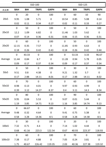
Table 2 - Comparison of results in Taillard´s testbed SSD-100 and SSD-125 (Makespan)
SSD-100 SSD-125
n x m BAH BIH TRIPS GAPH BAH BIH TRIPS GAPH
20x5
0 20 0 100 0 60 10 90
9.95 1.08 5.71 0 10.54 0.85 5.08 0.14
0.02 0.11 0.34 0.27 0.02 0.11 0.33 0.27
20x10
0 50 0 100 0 50 0 100
12.2 1.09 6.82 0 11.46 1.03 5.62 0
0.07 0.14 0.36 0.31 0.06 0.15 0.36 0.31
20x20
0 60 0 100 0 50 0 100
12.15 0.35 7.57 0 11.85 0.93 6.63 0
0.18 0.26 0.42 0.43 0.18 0.26 0.42 0.44
Average
0 43.33 0 100 0 53.33 3.33 96.67
11.44 0.84 6.7 0 11.28 0.94 5.78 0.05
0.09 0.17 0.37 0.34 0.09 0.17 0.37 0.34
50x5
0 50 0 100 0 30 0 100
9.51 0.8 4.38 0 9.21 1.32 5.7 0
0.17 2.88 14.11 8.01 0.17 2.88 14.11 8.02
50x10
0 70 0 100 0 60 0 100
8.98 0.13 4.01 0 9.97 0.93 4.99 0
0.39 3.12 14.27 8.37 0.4 3.11 14.3 8.34
50x20
0 80 0 100 0 90 0 100
9.95 0.04 5.53 0 9.07 0.01 5.44 0
1.19 3.85 14.71 9.13 1.16 3.85 14.74 9.13
Average
0 66.67 0 100 0 60 0 100
9.48 0.32 4.64 0 9.41 0.75 5.38 0
0.58 3.28 14.36 8.5 0.58 3.28 14.38 8.5
100x5
0 30 0 100 0 20 0 100
7.32 0.71 4.4 0 7.14 1.02 4.44 0
0.68 41.16 223.3 122.54 0.67 40.93 223.37 118.93
100x10
0 60 0 100 0 70 0 100
7.38 0.17 4.88 0 7.05 0.24 3.81 0
100x20
0 70 0 100 0 90 0 100
8.05 0.37 5.37 0 6.82 0.08 4.47 0
5.18 43.87 228.77 123.35 5.19 44.09 229.54 123.4
Average
0 53.33 0 100 0 60 0 100
7.58 0.42 4.89 0 7 0.44 4.24 0
2.54 41.9 226.16 121.75 2.63 41.8 226.76 120.55
200x10
0 40 0 100 0 30 0 100
6.37 0.59 4.21 0 5.59 0.56 3.44 0
6.87 613.21 3780.1 1853.66 7.03 618 3793.94 1836.08
200x20
0 60 0 100 0 60 0 100
6.55 0.09 3.45 0 5.7 0.09 3.15 0
21.19 632.35 3657.28 1846.33 21.13 633.6 3649.61 1844.22
Average
0 51.11 0 100 0 50 0 100
6.83 0.36 4.18 0 6.1 0.36 3.61 0
10.2 424.95 2554.51 1273.91 10.26 424.02 2556.77 1266.95
One interesting characteristics from the experimental analysis is that the methods seem to be unaffected by distribution of processing or setup times, i.e., there are no better methods depending on the specific distribution of processing or setup times.
Comparing GAPH with BIH, we observe that GAPH always gets equal or better results than BIH. The minimum success rate of GAPH was 90%, while the minimum of BIH was 20%.
With respect to the CPU time, TRIPS require much more
computational effort than GAPH and BIH. As it can be observed in Tables 1 and 2, for the biggest problem analyzed (200x20), the average CPU time of TRIPS was nearly 3660s, while TRIPS required nearly 630s and GAPH required nearly
1850s.
Finally, our proposal heuristic is statistically better than the rest of the heuristics, although it is more time consuming than BIH. GAPH always gets the better result, and is more efficient than TRIPS.
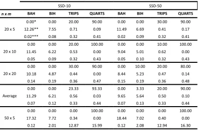
Table 3 - Comparison of results in Taillard´s testbed SSD-10 and SSD-50 (Total Flowtime)
SSD-10 SSD-50
n x m BAH BIH TRIPS QUARTS BAH BIH TRIPS QUARTS
20 x 5
0.00* 0.00 20.00 90.00 0.00 0.00 30.00 90.00
12.26** 7.55 0.71 0.09 11.49 6.69 0.41 0.17
0.02*** 0.08 0.32 0.41 0.02 0.09 0.32 0.41
20 x 10
0.00 0.00 20.00 100.00 0.00 0.00 10.00 100.00
11.45 6.22 0.53 0.00 9.04 5.01 0.62 0.00
0.05 0.09 0.32 0.43 0.05 0.10 0.32 0.43
20 x 20
0.00 0.00 30.00 90.00 0.00 10.00 20.00 80.00
10.18 4.87 0.44 0.00 8.44 5.23 0.47 0.14
0.14 0.19 0.36 0.47 0.15 0.19 0.36 0.48
Average
0.00 0.00 23.33 93.33 0.00 3.33 20.00 90.00
11.29 6.21 0.56 0.03 9.65 5.64 0.50 0.10
0.07 0.12 0.33 0.44 0.07 0.13 0.33 0.44
50 x 5
0.00 0.00 0.00 100.00 0.00 0.00 0.00 100.00
17.32 7.72 0.34 0.00 18.44 7.02 0.40 0.00
50 x 10
0.00 0.00 0.00 100.00 0.00 0.00 20.00 80.00
20.24 7.90 0.39 0.00 17.64 6.90 0.24 0.11
0.31 2.35 13.00 16.65 0.31 2.27 13.07 16.75
50 x 20
0.00 0.00 0.00 100.00 0.00 0.00 0.00 100.00
18.51 6.95 0.68 0.00 17.08 6.07 0.64 0.00
0.92 2.86 13.98 16.91 0.91 2.84 14.27 17.16
Average
0.00 0.00 0.00 100.00 0.00 0.00 6.67 93.33
18.69 7.52 0.47 0.00 17.72 6.66 0.43 0.04
0.45 2.41 13.28 16.52 0.45 2.40 13.43 16.74
100 x 5
0.00 0.00 0.00 100.00 0.00 0.00 0.00 100.00
22.93 8.11 0.27 0.00 24.94 6.85 0.17 0.00
0.50 32.12 217.34 258.54 0.51 32.78 215.95 259.79
100 x 10
0.00 0.00 0.00 100.00 0.00 0.00 0.00 100.00
24.09 7.20 0.52 0.00 21.25 6.14 0.46 0.00
1.25 33.01 216.13 265.60 1.26 32.48 216.72 265.86
100 x 20
0.00 0.00 10.00 90.00 0.00 0.00 10.00 90.00
25.07 6.06 0.36 0.21 20.88 5.07 0.26 0.04
3.70 35.35 218.32 265.61 3.72 35.70 218.47 268.15
Average
0.00 0.00 3.33 96.67 0.00 0.00 3.33 96.67
24.03 7.12 0.39 0.07 22.36 6.02 0.30 0.01
1.82 33.49 217.26 263.25 1.83 33.65 217.05 264.60
200 x 10
0.00 0.00 0.00 100.00 0.00 0.00 0.00 100.00
28.80 6.27 0.21 0.00 26.12 5.47 0.34 0.00
5.15 511.98 3494.11 4133.52 5.17 513.02 3490.31 4130.08
200 x 20
0.00 0.00 10.00 90.00 0.00 0.00 0.00 100.00
31.86 6.04 0.13 0.04 27.83 5.83 0.09 0.00
14.90 515.71 3537.08 4164.64 14.82 515.82 3517.09 4158.26
Average
0.00 0.00 5.00 95.00 0.00 0.00 0.00 100.00
30.33 6.16 0.17 0.02 26.97 5.65 0.22 0.00
10.03 513.85 3515.60 4149.08 10.00 514.42 3503.70 4144.17
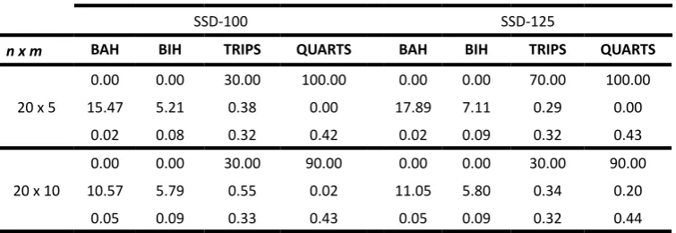
Table 4 - Comparison of results in Taillard´s testbed SSD-100 and SSD-125 (Total Flowtime)
SSD-100 SSD-125
n x m BAH BIH TRIPS QUARTS BAH BIH TRIPS QUARTS
20 x 5
0.00 0.00 30.00 100.00 0.00 0.00 70.00 100.00
15.47 5.21 0.38 0.00 17.89 7.11 0.29 0.00
0.02 0.08 0.32 0.42 0.02 0.09 0.32 0.43
20 x 10
0.00 0.00 30.00 90.00 0.00 0.00 30.00 90.00
10.57 5.79 0.55 0.02 11.05 5.80 0.34 0.20
20 x 20
0.00 0.00 40.00 90.00 0.00 0.00 10.00 100.00
8.57 4.66 0.34 0.00 8.96 4.54 0.32 0.00
0.14 0.20 0.36 0.47 0.14 0.20 0.36 0.48
Average
0.00 0.00 33.33 93.33 0.00 0.00 36.67 96.67
11.54 5.22 0.43 0.01 12.63 5.82 0.32 0.07
0.07 0.12 0.34 0.44 0.07 0.13 0.33 0.45
50 x 5
0.00 0.00 10.00 100.00 0.00 0.00 60.00 70.00
25.77 7.76 0.29 0.00 27.32 8.15 0.24 0.46
0.12 2.04 12.97 16.67 0.13 2.05 12.96 16.55
50 x 10
0.00 0.00 0.00 100.00 0.00 0.00 0.00 100.00
19.1 6.58 0.24 0.00 19.69 6.80 0.30 0.00
0.31 2.29 13.11 16.82 0.31 2.22 13.10 16.93
50 x 20
0.00 0.00 0.00 100.00 0.00 0.00 0.00 100.00
16.28 4.78 0.30 0.00 15.37 4.83 0.24 0.00
0.92 2.87 14.26 17.25 0.92 2.85 14.10 17.47
Average
0.00 0.00 3.33 100.00 0.00 0.00 20.00 90.00
20.38 6.37 0.28 0.00 20.79 6.59 0.26 0.15
0.45 2.40 13.45 16.91 0.45 2.37 13.39 16.98
100 x 5
0.00 0.00 0.00 100.00 0.00 0.00 30.00 100.00
30.5 6.37 0.13 0.00 33.78 6.68 0.05 0.00
0.50 33.21 215.57 265.68 0.51 32.97 218.75 267.20
100 x 10
0.00 0.00 0.00 100.00 0.00 0.00 10.00 90.00
23.51 5.69 0.16 0.00 23.67 6.08 0.12 0.06
1.27 32.70 217.09 269.60 1.27 32.78 217.73 271.06
100 x 20
0.00 0.00 0.00 100.00 0.00 0.00 0.00 100.00
19.67 4.71 0.22 0.00 18.91 4.27 0.16 0.00
3.71 34.97 219.34 269.38 3.72 35.02 218.98 270.50
Average
0.00 0.00 0.00 100.00 0.00 0.00 13.33 96.67
24.56 5.59 0.17 0.00 25.45 5.68 0.11 0.02
1.83 33.63 217.33 268.22 1.83 33.59 218.48 269.58
200 x 10
0.00 0.00 20.00 80.00 0.00 0.00 0.00 100.00
27.88 5.17 0.07 0.04 28.71 5.69 0.05 0.00
5.18 511.11 3502.32 4158.17 5.15 512.84 3522.19 4165.47
200 x 20
0.00 0.00 0.00 100.00 0.00 0.00 20.00 80.00
24.30 5.27 0.09 0.00 24.30 5.27 0.09 0.00
14.91 514.98 3528.10 4166.21 14.87 515.03 3518.97 4178.01
Average
0.00 0.00 10.00 90.00 0.00 0.00 10.00 90.00
26.09 5.22 0.08 0.02 26.50 5.48 0.07 0.00
As can be seen from the results in Tables 3 and 4, QUARTS heuristic obtains better results than the rest of the constructive heuristics. The success rate of QUARTS is superior to all heuristics, in all problems tested. QUARTS obtained the best solution in 95.23% of all problems tested, while TRIPS only obtained the best solution in 12.27% of them. We observed that TRIPS success rate decays with the increase of the number of jobs, indicating that this method works better for small problems. BAH and BIH are
not competitive with the other heuristics tested. All success rates for BAH were zero, and BIH only got the best solution
once.
Considering the ARPD, BAH has the highest values. Its ARPD exceeds 30% in some cases. The second method with the highest ARPD is BIH, with an ARPD of 5% in average. Analyzing TRIPS, we can see that its higher ARPD is 0.71%, and its ARPD average is 0.31%. Despite TRIPS success rate decays with the increase of jobs, its ARPD shows that the method gets better results with the increase of jobs. Its ARPD decays with the increase of jobs. The ARPD analysis ratifies the superiority of QUARTS, regarding the solution quality. Its ARPD average is 0.04%, about 8 times lower than TRIPS.
With respect to the CPU time, BAH is the fastest method, followed by BIH. The average CPU time of BAH was about 2.5s, while BIH required nearly 104s. Comparing TRIPS and QUARTS, we can see that TRIPS is a little faster than QUARTS. The average CPU time of TRIPS was about 702s, while QUARTS required 833s. As we can see in Tables 3 and 4, the CPU time of both methods always have the same order of precision. So, the difference between them is not significant. Finally, among the four methods evaluated in this computational experiment for the total flow time criteria, we can see that QUARTS is the better one, regarding the solution quality. In average, its success rate is 95.10% and its ARPD is 0.04%, while the methods BAH, BIH and TRIPS have success rates of 0%, 0.23% and 12.27% and ARPDs of 19.93%, 6.10% and 0.31%, respectively. With respect to the CPU time, although TRIPS is a little bit faster than QUARTS, this difference is insignificant. Thus, we can conclude that QUARTS is the better constructive heuristic for the total flow time criteria.
CONCLUSION
In this paper, we dealt with the problem of scheduling
a no-wait flow shop with sequence-dependent setup times with both make span and total flow time objectives by means of constructive heuristics. We presented two new heuristics, named GAPH and QUARTS, for the make span and total flow time criteria, respectively, and carried out extensive computational experiment. The results showed that GAPH
and QUARTS get better results than the other constructive heuristics tested. Henceforth, it can be concluded that the proposed heuristics obtain high solution quality comparing to the existing constructive heuristics for the problems, in acceptable computational times.
ACKNOWLEDGMENT
The research of the first author is partially supported by The State of São Paulo Research Foundation (FAPESP)
under grant number 09/06832-2. The research of the second author is partially supported by a grant number 473654/2009-1 from the National Council for Scientific and Technological Development(CNPq), Brazil.
REFERENCES
Aldowaisan, T. (2001). A new heuristic and dominance relations for no-wait flowshops with setups, Computers &
Operations Research, 28 (6), 563-584.
Allahverdi, A. & Aldowaisan, T. (2001). Minimizing total completion time in a no-wait flowshop with sequence-dependent additive changeover times, Journal of the
Operational Research Society, 52 (4), 449-462.
Allahverdi, A., Ng, C.T., Cheng, T.C.E. & Kovalyov, M.Y. (2008). A survey of scheduling problems with setups times
or costs, European Journal of Operational Research, 187 (3),
985-1032.
Allahverdi, A. & Soroush, H.M. (2008). The significance of reducing setup times/setup costs, European Journal of
Operational Research, 187 (3), 978-984.
Bianco, L., Dell’Olmo, P. & Giordani, S. (1999). Flow shop no-wait scheduling with sequence-dependent setup times
and release dates, INFOR Journal, 37 (1), 3-19.
Brown, S.I., Mcgarvey, R. & Ventura, J.A. (2004). Total flowtime and makespan for a no-wait m-machine flowshop with set-up times separated, Journal of the Operational Research Society, 55 (6), 614-621.
França, P.M., Tin Jr, G. & Buriol, L.S. (2006). Genetic Algorithms for the no-wait flowshop sequencing problem with time restrictions, International Journal of Production Research, 44 (5), 939-957.
Gupta, J.N.D. (1986). Flowshop schedules with sequence-dependent setup times, Journal of Operations Research Society of Japan, 29 (3), 206-219.
Ruiz, R., Maroto, C. & Alcaraz, J. (2005). Solving the
flowshop scheduling problem with sequence-dependent setup times using advanced metaheuristics, European
Stafford Jr, E.F. & Tseng, F.T. (1990). On the Srikar-Ghosh MILP model for the NxM SDST flowshop problem,
International Journal of Production Research, 28 (10), 1817-1830.
Stafford Jr, E.F. & Tseng, F.T. (2002). Two models for a family of flowshop sequencing problems, European Journal
of Operational Research, 142 (2), 282-293.
Taillard, E. (1993). Benchmarks for basic scheduling
problems, European Journal of Operational Research, 64 (2),