In Situ Observations of Pearl Pulsations and Development of a Low-Noise Fluxgate Magnetometer, Kristoff Paulson

(1)

University of New Hampshire

University of New Hampshire Scholars' Repository

Doctoral Dissertations

Student Scholarship

Winter 2018

In Situ Observations of Pearl Pulsations and

Development of a Low-Noise Fluxgate

Magnetometer

Kristoff Paulson

University of New Hampshire, Durham

Follow this and additional works at:

https://scholars.unh.edu/dissertation

This Dissertation is brought to you for free and open access by the Student Scholarship at University of New Hampshire Scholars' Repository. It has been accepted for inclusion in Doctoral Dissertations by an authorized administrator of University of New Hampshire Scholars' Repository. For more information, please [email protected].

Recommended Citation

Paulson, Kristoff, "In Situ Observations of Pearl Pulsations and Development of a Low-Noise Fluxgate Magnetometer" (2018). Doctoral Dissertations. 2427.

(2)

In situ observations of pearl pulsations and

development of a low-noise fluxgate magnetometer

BY

KRISTOFF PAULSON

B.A. in Physics, Religious Studies - Colby College, 2006

DISSERTATION

Submitted to the University of New Hampshire

in partial fulfillment of

the requirements for the degree of

Doctor of Philosophy

in

Physics

(3)

This dissertation was examined and approved in partial fulfillment of the requirements for the degree of Doctor of Philosophy in Physics by:

Dissertation Director, Roy Torbert, Professor of Physics, UNH

Charles Smith, Professor of Physics, UNH

Marc Lessard, Professor of Physics, UNH

Mark Engebretson, Professor of Physics, Augsburg College

Karsten Pohl, Professor of Physics, UNH

On October 29th_{, 2018}

(4)

Acknowledgments

This work was supported by Iowa subcontract 1000556126 to UNH in support of the Van

Allen Probes spacecraft and EMFISIS/MAG instruments and by NSF at UNH under grants

PLR-1141987 and AGS-1202827. Additional support was provided by NASA through NASA Space Grant

Fellowship NNX15AH79H. The Ming/Chen scholarship and several UNH travel grants provided the

funding necessary to discuss these results with the international space science community at various

conferences and meetings.

To the members of my committee, thank you for providing me with the guidance and

indepen-dence (as well as the patience) to let me explore the world of space science. I have been exposed

to a multitude of different areas of the plasma physics field by working with each of you on many

different projects, and I am extremely grateful to have been able to experience so many fascinating

subjects.

I am indebted to all of the professors and colleagues I have worked with at UNH who have all

been generous and willing in their assistance. In particular, I would like to thank Matthew Argall

and Sam Bingham who have helped me work through much of the derivation and analysis used in

this study.

I am also grateful to Jeremy Faden, whose Autoplot software was used to generate the majority

of figures herein.

Most importantly, I would like to thank my wife Tara for supporting my gambit to spend years

looking at space data. Her determination and passion for her own work have been an inspiration to

help guide me through this process, and I would not have been able to finish without her support

(5)

List of Tables

1.1 Period and Frequency range of geomagnetic pulsations in the ULF range as defined

by IAGA . . . 4

3.1 Calibration parameters satisfying eqs (3.3) determined from comparisons between

measured field and IGRF-12 model. . . 53

3.2 Angles making up rotation from the instrument to spacecraft coordinate system. . . 55

5.1 Wave Events with Periodically Oscillating Poynting Flux . . . 114

(10)

List of Figures

2-1 Two versions of the basic rod-core magnetometer sensor design . . . 22

2-2 Construction of a ring-core magnetometer . . . 22

2-3 Depiction of standardized hysteresis curve . . . 24

2-4 Fluxgate magnetometer input and sensed waveform examples . . . 27

2-5 Permalloy grain size comparison for different heat treatment processes . . . 29

2-6 Diagram of a fluxgate magnetometer with racetrack geometry . . . 31

3-1 Coefficients of expansion . . . 35

3-2 Racetrack bobbin model . . . 36

3-3 Racetrack sensor heat treatment profile . . . 37

3-5 RENU2 racetrack magnetometer sensor . . . 38

3-6 Racetrack magnetometer sensor noise calculation . . . 39

3-7 RENU2 racetrack magnetometer exploded diagram . . . 40

3-8 Racetrack magnetometer mounted on RENU2 . . . 41

3-4 Racetrack sensor model . . . 41

3-9 RENU2 racetrack magnetometer mag-cal results . . . 42

3-10 Non-orthogonal axis diagram . . . 45

3-11 RENU2 racetrack magnetometer raw measurements . . . 47

3-12 Telemetry stream for racetrack magnetometer showing anomalous data . . . 48

3-13 Racetrack magnetometer spin axis offset drift correction . . . 50

3-14 Racetrack magnetometer data pre-calibration . . . 51

3-15 Racetrack magnetometer residue field . . . 52

3-16 Racetrack magnetometer data post-calibration . . . 52

3-17 Spectral Power of Racetrack Magnetometer Before Alignment . . . 53

(11)

4-1 Wave resonance boundaries . . . 64

4-2 Dispersion relation for transverse wave . . . 70

4-3 Dispersion relation for compressional wave . . . 74

4-4 Comparison between unstructured EMIC wave and Pc1 Pearl Pulsation . . . 78

4-5 Original observations of Pc1 pearl events . . . 79

4-6 Classifications of Pc1 wave modes from spectral characteristics . . . 81

4-7 Conjugate ground-based Pc1 pearl pulsation observations . . . 84

4-8 Eigenmodes of cyclotron resonator harmonics . . . 87

5-1 Van Allen Probes observation coverage during study . . . 92

5-2 Example of EMIC wave selection . . . 99

5-3 Spatial occurrence and wave power distributions of EMIC waves in MLT . . . 100

5-4 Spatial occurrence distributions of EMIC waves in MLat . . . 103

5-5 Spatial extent distributions of EMIC wave events . . . 104

5-6 Temporal separation of multipoint EMIC wave events . . . 105

5-7 Distribution of wave events by storm phase . . . 107

5-8 Distribution of wave events from Dst minimum . . . 108

5-9 Distribution of wave observations by geomagnetic activity indices . . . 110

5-10 Example wave event showing alternating Poynting Flux propagation . . . 112

5-11 Pearl pulsation observation examples relative to plasmapause . . . 115

5-12 Example of normalized frequency fits . . . 117

5-13 Distribution of slopes of wave event frequency-L fits . . . 118

5-14 Van Allen Probes magnetic footpoint locations for 2012-09-10 event . . . 119

5-15 Conjugate wave spectrograms for 2012-09-10 event . . . 120

5-16 Polarization analysis for 2012-09-10 event . . . 121

5-17 Van Allen Probe-B magnetic footpoint location for 2012-11-11 event . . . 122

5-18 Conjugate wave spectrograms and ellipticity for 2012-11-11 event . . . 123

5-19 Conjugate integrated wave power enhancements for 2012-11-11 event . . . 124

(12)

6-2 Comparison of observed pearl modulation frequency to calculated BWP reflection

frequency . . . 129

6-3 Frequency structure of individual pearl element . . . 132

6-4 MMS spectrograms of pearl pulsation event on 2015-06-25 showing relation to plasma-pause boundary . . . 138

6-5 MMS spectrograms of Pearl pulsation event on 2015-06-25 highlighting simultaneous pearl elements . . . 139

6-6 Wave power at two frequency bands for 2015-06-25 event . . . 141

6-7 Wave properties for 2015-06-25 event . . . 142

6-8 Wave properties for 2013-03-20 event . . . 145

6-9 Particle and wave data for 2013-03-20 event . . . 147

6-10 Horizontal and vertical power slices of 2013-03-20 event. . . 148

6-11 Example of beating pattern created by harmonic waves . . . 150

6-12 Plasma boundaries identified by algorithm . . . 152

6-13 Distribution of plasma boundaries . . . 154

6-14 Wave power sorted by plasma boundary . . . 155

(13)

ABSTRACT

In situ observations of pearl pulsations and development of a low-noise

fluxgate magnetometer

by

Kristoff Paulson

University of New Hampshire

This work is comprised of two main efforts: the design, construction, and flight of a rocket-borne

fluxgate magnetometer, and the examination of Pc1 pearl pulsations using data from the Van Allen

Probes and MMS missions.

Our first concentration regards the design and fabrication of an improved fluxgate

magnetome-ter. The instrument makes use of an elongated racetrack geometry to improve on the signal-to-noise

ratio of previous designs. We additionally examined refined heat treatment procedures to optimize

the crystal structure of the magnetically permeable core material and were able to increase the size

of crystal grains. The magnetometer was successfully flown on the RENU2 auroral sounding rocket

mission, although the recorded data were coarser than would allow for current identification. We

go on to demonstrate the methods employed to perform a flight orthogonalization and calibration

of the instrument using comparisons of the measured field to the modeled IGRF field.

Our second effort concerns the in situ examination of Pc1 pearl pulsations using data from

the Van Allen Probes and MMS missions. These waves were found to differ from traditional

unstructured EMIC waves in their spatial and storm-time occurrence, as well as in the independence

of their excitation frequency relative to the background magnetic field. This independence, as

well as conjugate observations showing similar behavior in space and on the ground, contradicts

previously proposed generation mechanisms. We found a dependence of both occurrence and wave

(14)

magnetosphere near the plasmapause. Additionally, we recorded cases of pearl pulsation events

alternately displaying the characteristics of magnetosonic and ion cyclotron waves. We propose

that pearl pulsations are generated through the coupling of incident magnetosonic wave energy

with the ion cyclotron wave mode at the dispersion surface created by this heavy ion boundary.

Closely-spaced harmonics of wave activity in the magnetosonic mode would constructively interfere

(15)

Chapter 1 Introduction

The interaction between transient disturbances launched from the Sun and the Earth’s magnetic

field provide a wealth of energetic processes and particle populations. These can range from sudden

injections of energy, such as the hour-long substorms which drive the night time aurora, to the

formation of belts of highly energetic particles, which can persist for months.

The framework that holds this system together and allows these different processes to interact

is the magnetic field generated at the Earth’s core. The transfer of energy to different parts of

this framework is mostly accomplished through the generation and propagation of electromagnetic

waves. These waves come in many different flavors, and are most often categorized by their

direc-tion of propagadirec-tion, polarizadirec-tion, and frequency range. We can detect these waves in the Earth’s

magnetosphere by measuring deviations/fluctuations in both the magnetic and electric fields.

Ad-ditionally, in order to characterize the directionality and polarization of the wave, we must be able

to measure the strength and direction of the background magnetic field. The instrument most

commonly used to perform this function in the space environment is the fluxgate magnetometer.

The first half of this study will describe our work on the development and construction of an

improved fluxgate magnetometer design called a racetrack magnetometer. In the second half we will

examine a particular subset of electromagnetic ion cyclotron waves known as Pc1 pearl pulsations,

which are responsible for the energy transfer between resonant ion populations (and possibly to

(16)

1.1 What is a Space Plasma?

The medium that fills the interplanetary space outside of Earth’s atmosphere consists of a plasma.

Sometimes referred to as a fourth state of matter (beyond the traditional phases of solid, liquid,

and gas), a plasma is an energetic state of matter that behaves in many ways like a fluid, but is

composed of electrically charged particles. The electrical charge typically results from the stripping

away of one or more electrons from the neutral particle by sufficiently energetic photons or

charge-exchange collisions. Due to their charge, these particles are additionally constrained by any present

magnetic (and possibly electric) field. Whether the motion of the magnetic field dominates the

motion of the particles or vice versa depends on the ratio of the plasma particle pressure to the

magnetic field pressure given by β = (nkBT)/(B2/2µ0). Where the particle pressure dominates

that of the magnetic field (ie, high densitynor average temperatureT), the motion of the particles

will drag the field with it, in turn influencing the motion of surrounding particles interacting with

the same field line. Where the magnetic pressure dominates (ie, high magnetic field strength B),

the motion of field lines will push and pull nearby particles along.

Plasmas can be created in laboratory environments seeking to study subjects such as fusion

and manufacturing, but the plasma that exists in outer space differs by its extremely low density.

While this region does not constitute a perfect vacuum, the density of the interplanetary space

environment is several orders of magnitude smaller than that achievable in a laboratory. In the

near-Earth solar wind, for example, a typical pressure measurement is on the order of several

nanoPascals, whereas the lowest value attained in typical laboratory pressure chambers is on the

order of1010 nanoPascals.

Because of this low density, space plasmas are often described as collisionless. In this

environ-ment, the rate at which ionized particles come into contact with stray electrons to recombine into

a neutral particle is so low that for the region and timescales we are interested in studying we can

(17)

equations of motion governed by electromotive forces. The ease of motion along a magnetic field

line, especially for electrons, means any field-aligned electric field structures are short-lived, and

the plasma takes on a neutral average charge density.

Towards lower altitudes at Earth, the magnetospheric environment transitions from a rarefied

space plasma to the dense neutral atmosphere near ground level. Within this transition region lies

the ionosphere, a range of the upper atmosphere composed of both ionized plasma and a larger

neutral population. While the ionized component still interacts with the background magnetic field

as described in section 1.3, the dominant neutral component reduces the mean free path length

traveled by ions and electrons before colliding with other particles. These collisions translate into

finite measurements of electrical conductivity/resistance as well as convection. By enabling finite

electrical conduction across the magnetic field, the ionosphere provides a source of current closure

for magnetospheric field-aligned currents and a distinct change in the refractive index for traveling

plasma waves.

The lack of collisions in the magnetosphere means that more familiar modes of energy

trans-fer1 are not available, which can lead to non-isotropic distributions of particle populations. These

can range from uneven distributions of temperatures in certain directions, to overlapping

popula-tions of different energy ranges, to isolated beams through a stationary group of particles. These

anisotropies in the plasma are still unstable configurations, however, as they would be in any

typ-ical fluid or particle distribution. To achieve a state of lowest potential energy, the system will

seek isotropization of these distributions, and will do so via a radiative transfer of energy and

momentum, ie wave generation.

(18)

Classification Period (sec.) Frequency (Hz)

Pc 1 0.2 to 5 0.2 to 5

Pc 2 5 to 10 0.1 to 0.2

Pc 3 10 to 45 0.022to 0.1 Pc 4 45 to 150 0.006to0.022

Pc 5 150 to 600 0.0016 to0.006

Pi 1: 1 to 40 sec 0.025 to 1 Pi 2: (primarily pt) 40 to 150 sec 0.006to 0.025

Table 1.1: Period and Frequency range of geomagnetic pulsations in the ULF range as defined by IAGA

1.2 Plasma Waves

The rarefied nature of a space plasma implies particles cannot exchange information through

col-lisions. This rules out the presence of collisional interactions such as traditional acoustic waves.

Instead, waves in this medium must propagate through the available field structures so will be

confined to electromagnetic and electrostatic modes, as well as the magnetosonic mode (a hybrid

version of a magnetic and acoustic wave mode). Electromagnetic wave modes can travel from the

space environment to the Earth’s surface where they can be detected by magnetic or electric field

oscillation measurement instruments. Because of this, most early studies of the magnetosphere

relied on inferences from wave observations made on the ground.

Plasma wave classifications were first made according to oscillation period, and were delineated

into strict categories by the International Association of Geomagnetism and Aeronomy (IAGA).

Table 1.1 lists the wave period and frequency ranges for continuous pulsations (Pc) and

irregu-lar pulsations (Pi) in the Ultra Low Frequency (ULF) range as defined by IAGA in Resolution

13 (1963). These somewhat arbitrary classifications provide little explanation into the driving

in-stability or wave mode, but are still used today in order to provide a reference to other known

frequencies and wave ranges.

The pearl pulsations we will primarily focus on in this work fall into the Pc1-2 range, but

(19)

of the electromagnetic ion cyclotron (EMIC) wave mode described in section 4, and are typically

generated through resonant interactions between field perturbations and the left handed cyclotron

motion of ions.

1.3 Particle Motion

There are three types of motion to describe the trajectory undertaken by a charged particle in

Earth’s magnetosphere: cyclotron gyration, field-aligned bounce, and orbital drift. These act in

concert to form a complicated orbit which can be disrupted by various external drivers depending

on the time and spatial scales affected.

1.3.1 Cyclotron Motion

The first type of particle motion, cyclotron gyration, describes the movement of a particle in the

presence of a static and homogeneous magnetic field. Plasma particles are primarily guided by the

Lorentz-force law

⃗

FL=q ⃗E + q ⃗v×B⃗ (1.1)

for an electric field E⃗, a magnetic field B⃗, particle charge q, and particle velocity ⃗v. Immediately

we can see from (1.1) that any electric fields oriented in the same direction as _B⃗ _{due to charge}

separations will quickly be counteracted by movement of the particle along (or against, depending

on the sign of q) the field direction. The second term, however, describes a force perpendicular to

both the particle motion and the magnetic field direction. What this means is that the component

of the particle velocity directed across the magnetic field will lead to the creation of a force turning

that particle’s motion. In the simplest case, the motion of the particle in the plane perpendicular to

(20)

for a component_⊥perpendicular to _B⃗ _{is given by}

FL⊥=mv˙⊥=qBv⊥

so that we are left with a circle traced out with the angular frequency

Ωc=

qB m

known as the cyclotron frequency. The gyrofrequency fc = Ωc/2π then is a particle property

independent of its kinetic energy or direction of motion (for the non-relativistic particles we will

consider here), and varying only by the strength of the local magnetic field measurement B. The

direction (or handedness) of this cyclotron motion will depend on the sign of the chargeq, and will

be right-handed for electrons, while left-handed for ions.

The differences in mass mean that the gyrofrequencies for electrons and protons will be separated

by an order of _∼1840. The mass mwill lead to lower cyclotron values for heavier ions such as He+

and O+_{, and though the number densities for doubly-ionized are typically low enough in Earth’s}

magnetosphere that we do not typically consider their contribution, the chargeq will give a higher

gyrofrequency for He++ _{than He}+_{. We will see in section 4.1 that disparity in cyclotron value will}

lead to wave modes in very different frequency regimes, and that wave modes in the Pc1-2 range

resonant with positively-charged particles will often be separated into bands based on the wave

frequency relative to local ion gyrofrequencies. The gyrofrequency of a proton will typically be on

the order of several Hz in our region of study, and this same gyromotion will constitute the resonant

(21)

1.3.2 Bounce Motion

The second type of particle motion relates to the motion of a charged particle within a magnetic

bottle. Rather than a homogeneous magnetic field as above, we will now consider this field to

exhibit a positive gradient in magnitude away from a midpoint. The particle will still undergo the

gyromotion, but as we saw in equation (1.1), the equation of motion leading to this gyration is only

due to the particle velocity perpendicular to_B⃗_{. If there is any parallel component to the particle}

velocity, this gyration will turn into a helical motion from a stationary point of view. In cases where

the field gradient is gradual (ie, small in relation to the total field over a single gyration orbit), the

particle’s magnetic moment

µ=

1 2mv

2

⊥

B

will be conserved [Northrop and Teller, 1960]. This moment µ is known as the first adiabatic

invariant, and the conditions of a gradual relative change inB are often conserved for geomagnetic

disturbances.

As the particle moves along the gradient to regions of larger magnitude, µwill be conserved, so

v_⊥2 must also increase. We have stated before that E_∥= 0 due to the fast motion of electrons along

the field to quench any induced electric field, and since the magnetic field does not accelerate the

particle the total kinetic energy will be conserved. For 1 2mv

2 _{to remain constant as} _v

⊥ increases,

v_∥ must decrease until it reaches a point where v_∥= 0. This is known as the mirror point, and the

particle will reflect from this point back towards the region of lower field magnitude, overshooting

and in turn being reflected at the opposite mirror point. Particles are thus trapped within this

magnetic bottle, reflecting back and forth while gyrating along the field lines.

In the dipolar magnetosphere, this bottle is generated by the increase of field strength at the

magnetic poles relative to the equatorial field magnitude. Particles gyrating about field lines will

(22)

value αeq = tan−1(v⊥/v∥) as measured at the magnetic equator, the typical point of minimum B

along a magnetic field line in a dipole configuration2). The typical timeframe of this bounce motion

for protons is on the order of minutes. Particles with higher energy and more field-aligned equatorial

pitch angle values will mirror at higher (ie, more poleward) magnetic latitudes, possibly reaching

a configuration where they encounter collisions with the neutral atmosphere close to the Earth’s

surface. These particles are then considered “lost” to the magnetospheric system. This process

is referred to as precipitation, and is driven by mechanisms which can violate the steady-state

requirements of the first adiabatic invariant such as wave-particle interactions.

The typical timescales of this bounce motion for ions is on the order of the temporal modulation

of pearl pulsations. This has led to several generation theories (discussed in section 4.3.1) which

tie the bounce motion of bunched particles and resonant waves with pearl modulation.

1.3.3 Drift Motion

The third type of particle motion relates to electric fields and forces oriented perpendicular to _B⃗_,

and leads to particle velocity across the field direction. This is known as the drift motion, and is

given by

vD =

⃗ E×B⃗

B2 +

W_⊥B⃗ × ∇B

qB3 +

2W_∥rˆc×B⃗

qRcB2

(1.2)

whereW_⊥ and W_∥ are the perpendicular and parallel particle energy,Rcis the radius of curvature

of the magnetic field line, andrˆcis the unit vector pointing outwards from the center of curvature.

The second and third terms in equation (1.2) make up the bulk of the drift velocity component,

and are often referred to together as the gradient-curvature drift. The curvature arises when we

take the magnetic bottle configuration leading to the bounce motion and bend it such that the

2_{The pitch angle distribution}

f(α)for a given particle population is most often found to be symmetric about 90◦

(indicating a perfectly trapped population) so that measurements of0◦< f(αeq)< δand180◦−δ < f(αeq)<180◦

(indicating particles lost to the atmosphere) are identical. The valueδ defines what is referred to as the loss cone,

(23)

high-field endpoints curve downwards towards the surface of the Earth. This curvature creates a

centrifugal force on the particle as it bounces along the field line acting outwards across the field

direction. The decrease in field magnitude radially from the center of the Earth creates a gradient

across this magnetic bottle. As the particle gyrates around the field line, the gradient across the

range of this gyroorbit will generate a difference in gyroradius from one side of the orbit to the

other. This gradient will be directed in the opposite direction as rˆc, such that both terms will be

oriented together. It is important to note that both of these terms are dependent on the particle

charge q, so ions and electrons will drift in opposite directions around the Earth (ions moving

westwards while electrons move eastwards). This will lead to the generation of a portion of the

ring current described in section 1.4.2.

The first term in equation (1.2) is the basic _E⃗ _×_B⃗ _{drift motion for large-scale electric fields,}

and will incorporate contributions from the convection electric field (pointing from dawn to dusk)

generated by the constant stream of solar wind particles across Earth’s magnetosphere, and the

corotation electric field generated by the plasmaspheric plasma rotating with the diurnal motion

of the Earth. Both electrons and positive ions will travel eastwards, and there is no dependence

on particle energy or mass. This component is particularly important for lower energy ions, where

the _E⃗ _×_B⃗ _{drift can become comparable to the gradient-curvature drift. Simulations by} _Ferradas

et al. [2016] using realistic conditions show that for ions at energies less than ∼10 keV, the E⃗ ×B⃗

drift term can dominate. This eastward motion can contribute to the injection of lower-energy

ions across the dawn side of the magnetosphere into the morning sectors within tens of hours of

storm-driven particle injections.

1.3.4 Betatron Acceleration

Given the particle modes of motion described above, consider the case where the background

(24)

through compressions of the magnetosphere by solar wind transients or long period electromagnetic

waves in the Pc4-5 range or lower. By preserving the first adiabatic invariant, the perpendicular

component of the particle velocity will change in proportion to the magnetic field strength. This

process, known as betatron acceleration, will not conserve total kinetic energy, nor will it affect

the parallel velocity component. Instead, the equatorial pitch angle will focus towards 90◦ causing

the affected particle population to mirror at points closer to the magnetic equator. We will see

in section 4.2 that this mechanism can lead to instability conditions of free energy that is then

released in the form of electromagnetic waves such as the EMIC waves that make up our study.

1.4 Magnetosphere

The Earth’s magnetic field serves to mitigate impacts from disturbances in the solar wind. This

dynamic and reactive cavity is known as the Magnetosphere. The outward pressure exerted by the

primarily dipolar internal field is matched at some distance away from the Earth by a combination

of the particle pressure and interplanetary magnetic field pressure within the solar wind. The solar

wind pressure compresses the field on the sunward side of the magnetosphere creating a more oblate

shape, but in the inner magnetosphere where we have conducted the majority of our observations,

a dipole approximation is sufficient. This field is given as a function of the equatorial distance of

the field line from the center of the Earth r and the magnetic latitude (MLat) λby

B(r, λ) =B_⊕r

3

⊕

r3

√

1 + 3 sin2λ

cos6_λ (1.3)

whereB_⊕is the equatorial magnetic field strength at the Earth’s surface and r_⊕= 6371km is the

radius of the Earth. In these coordinates, the bounce motion described by particles gyrating along

field lines confines them to shells at a distance r =Lcos2λfrom the center of the Earth. The L

(25)

motion is often described in terms of motion along these Lshells, and magnetospheric regions are

often identified by their distance in L and the MLatλ[McIlwain, 1961].

A portion of the energy imparted from the collision of transient solar wind disturbances with

this magnetosphere is absorbed into the system through the generation of waves and the heating of

various particle populations. These processes, coupled with the constant barrage of solar radiation

and leakage of the upper atmosphere out into space, create a dynamic environment populated by

distinct particle populations.

The densities of these populations are rarefied to such an extent that in some regions these

populations will overlap in space without coming into direct contact. These populations cannot

come to a common equilibrium in terms of temperature or pitch angle distribution through the

direct interactions (ie, collisions) we observe in a traditional medium, so can only transfer energy

and information through a common shared structure. As explained in section 1.1, this structure is

the surrounding magnetic field.

1.4.1 Radiation Belts

The radiation belts, also known an as the Van Allen radiation belts, are two naturally-occurring

structures composed of high-energy particles in the inner to middle magnetosphere. Due to the

three methods of particle motion listed in section 1.3, these belts take on a toroidal shape as the

particles bounce between conjugate points and drift around the equator. They consist of an inner

belt at L=1.5-2 composed mostly of energetic (_∼10 MeV to 1 GeV) protons and an outer belt at

L=3-6 of high-energy (200keV to 10s of MeV) electrons. The inner belt is considered to be very

stable, with few geomagnetic disturbances able to affect its extent and plasma composition.

The outer belt, however, is highly dynamic and is both a driver and result of geomagnetic

processes. The inner limit of this belt is thought to be relatively stable, but differs in location

(26)

magnetopause during severe magnetic compressions, and the entirety of the belt can be lost to

magnetopause shadowing during the most extreme events. Similarly, the strength of the belt can

be increased or depleted following a storm due to a complex cascade of wave-particle interactions

that is still not fully understood.

The waves that are most commonly believed to be responsible for this electron energization are

a combination of whistler mode chorus waves and plasmaspheric hiss, though the magnetosonic

mode has also been shown to alter pitch angle configurations. EMIC waves have been theorized to

play a role in the depletion of these highest energy electrons through a Doppler shift of the observed

wave polarization when electrons move at relativistic speeds [Omura and Zhao, 2012;Denton et al.,

2015]. These revelations have renewed interest in the study of EMIC waves during the current era

of regular in situ measurements of radiation belt activity, especially for those waves exhibiting the

coherent rising frequency tones thought best able to trap relativistic electrons [Pickett et al., 2010;

Omura et al., 2010].

1.4.2 Ring Current

Further inwards than the outer reaches of the radiation belts, but overlapping in space lies the ring

current. This toroidal structure consists of an energetic plasma component in the 10-200 keV energy

range made up of both ions and electrons, and spans an Lshell range of ∼2-7. The particles at

this energy are dominated by the gradient-curvature drift terms, and so drift in opposite directions

around the Earth creating a current. This current structure induces a dipole magnetic field which

opposes the natural core-driven field.

The ring current is made up of both a stable and a storm-time component, so varies in

inten-sity relative to geomagnetic activity. The magnitude of this change is reflected in the Dst index,

described in section 1.5. The stable quiet-time ring current is generated by the net gyromotion

(27)

gyro-motion constitutes individual magnetic moments µ from which we can take a curl to find the net

magnetization currentJM:

jM =∇ ×(n+µ++n−µ−) =−∇ ×p⊥

(

⃗ B B2

)

.

Here we have translated the magnetic moment into the perpendicular pressure term p_⊥ via the

perpendicular velocity constituting gyromotion. Distributing the curl ultimately results in a

mag-netization current of the form

jM =

⃗ B

B2 × ∇p⊥ − 2p⊥

⃗

B× ∇B

B3 − p⊥

∇ × ∇_B⃗

B2

.

The particle motion described by the gradient and curvature drift velocities given by the second

and third terms in (1.2) can also be rewritten in terms of the perpendicular and parallel pressure

terms. Combining these withjM to form the total ring currentjrc, we find

jrc= ⃗ B

B2 ×

(

∇p_⊥+p∥−p⊥

B2 (B⃗ · ∇)B⃗

)

.

(1.4)

The storm-time portion of the ring current is formed by freshly injected particles from the

magnetospheric tail brought in by substorms as well as electric-field driven convective motion. It

coalesces over a period of hours, first forming a partial structure which eventually creates a complete

ring as particles drift around the Earth.

The ions that make up this current have a considerable amount of free energy, and are often

focused into a more trapped distribution through the betatron acceleration mechanism as they

are brought from low magnetic field regions in the tail to the inner magnetosphere. Additionally,

(28)

they will take slightly different drift paths based on their pitch angle. This “drift-shell splitting”

[Sibeck et al., 1987] results in distinct regions of higher temperature anisotropy as well as regions

comprising “butterfly” pitch angle distributions. These mechanisms form an unstable population of

anisotropic ions at 10s of keV which can most easily release their free energy through the generation

of ion cyclotron wave activity.

1.4.3 Plasmasphere

At lower Lshells than the higher-energy torii above, the corotating plasmasphere consists of dense

cold plasma in the _∼1 eV energy range. This region extends outwards from the tenuous upper

atmosphere near the surface of the Earth to a variable distance of L≃3-5 depending on geomagnetic

conditions. During active periods, the outer boundary can be eroded away through convection

driven by the solar wind [Nishida, 1966] over a period of several hours. During these periods, the

region previously dominated by the corotation electric field is taken over by the convection electric

field, pushing the dominance boundary to lower L. The convection field is oriented from Dawn to

Dusk across the magnetosphere, and accelerates plasma in the afternoon and dusk sectors outwards.

This creates a steep gradient in plasma density at this boundary known as the plasmapause roughly

circular in shape with an enhanced bulge at the dusk sector. As the geomagnetic storm progresses,

this bulge develops into a plume structure that extends sunward and wraps around the middle

magnetosphere. Over a period of several days after the main phase of the storm, the convection

boundary is reset to its original balanced configuration and plasma escaping along field lines from

the ionosphere refills the plasmasphere.

This dense plasma component is instrumental to the formation of various wave modes including

EMIC waves. For example, the plasmapause forms the boundary between regions of whistler mode

chorus and hiss wave growth (both electron-scale waves), and basic linear theory of ion cyclotron

(29)

at the plasmapause creates a change in the index of refraction for plasma waves altering their

propagation and polarization parameters. Localized flux tubes of relative high density act to

guide waves along the density enhancement, while rarefied tubes leak wave energy [Streltsov et al.,

2012]. Refractive surfaces will similarly be generated by transitions to regions of changing plasma

composition, since heavier ions will react differently to field perturbations. We will examine the

effects of such a surface where the O+ _{dominates over the H}+ _{for the 10s of keV energy range in}

the inner magnetosphere. We believe that this gradient in the EMIC wave dispersion surface is an

instrumental factor in the generation of Pc1 pearl pulsations.

1.4.4 Ionosphere

Finally, at the base of the plasmasphere and above the neutral atmosphere of the Earth is the

ionosphere. This is a dense region of plasma located at an altitude of 50-1000 km. This plasma is

formed by Solar UV radiation impinging on the local neutral particles and is mostly composed of

O+_{, especially at lower altitudes. This region allows for current closure for the field-aligned currents}

generated during storms and substorms, and the finite conductivity levels provide feedback to the

magnetosphere where they have an influence on the field structure and characteristics.

This highly conductive surface will not only affect the behavior of waves traveling through it

along field lines, but will generate a cavity known as the Alfvén Resonator Cavity allowing for

the ducting of waves along the Earth’s surface. This is particularly resonant with Pc1 waves, and

adds additional challenge to inferences of wave source regions made based on waves observed by

ground stations. As such, conjugate observations made between ground and in situ observatories

(30)

1.5 Solar Wind as a Driver

The constant barrage of energy from the Sun in the form of the Solar Wind is the primary driver of

activity and energization in the Earth’s magnetosphere. Not only does the incoming pressure warp

and compress the magnetic field structure, but the induced convection processes drive the flow of

magnetospheric plasma populations from the tail back into the inner magnetosphere. This constant

exchange of energy can only be isotropized in a collisionless medium through wave activity, so the

instabilities generated by this particle movement will inevitably lead to the generation of a cascade

of electromagnetic perturbations.

The basic cartoon of the geomagnetic storm generated by the interaction between the

magneto-sphere and a sudden pulse of pressure coupled with a southward-oriented interplanetary magnetic

field (IMF) is known as the Dungey Cycle [Dungey, 1961]. Incoming magnetic field with a

compo-nent anti-aligned with the Earth’s field will reconnect at the dayside, pushing back the outer reaches

of the magnetopause and connecting the magnetospheric cusp regions directly to the IMF. These

open field lines are swept back towards the tail with the flow of the solar wind, where a combination

of dynamic pressure and a generated tail current will once again lead to field line reconnection, this

time in the tail of the magnetosphere. The newly closed field line on the Earthward side of this

reconnection point will drag plasma from the tail region into the inner magnetosphere, where it

will either be lost to the atmosphere when accelerated by field-aligned currents or will be injected

into the ring current system.

Any increase in the strength of the ring current, also contributed to through global-scale

con-vection patterns, will oppose the Earth’s natural dipole field. This effect is measurable, and has

become a parameter by which the strength of these geomagnetic storms can be ranked known as the

disturbed storm time (Dst) index [Akasofu and Chapman, 1961]. The typical pattern of this index

is that an initially zero-valued Dst indicative of a stable ring current presence will initially rise by

(31)

known as the sudden commencement. The ring current will then be strengthened by incoming

energetic plasma, driving the Dst down to _∼-50 (for weak storms) or to _∼-400 nT (severe storms)

over a period of several hours. Over the next few days, the ring current energy will be lost to

particle scattering and wave generation, and the Dst will rise towards 0 nT. This typically happens

in two stages, with a faster early recovery period over the first 1-2 days followed by a late recovery

period spanning several days further. While a single measured value is incapable of describing the

myriads of small scale effects which may or may not occur during each storm, it does provide a

general idea of the severity and stage of the disturbance.

Two other indicators of geomagnetic activity are the K-index and the Auroral Electrojet Index.

The K-index is a quasi logarithmic conversion of disturbances of the horizontal magnetic field

component at various ground magnetometer stations into an integer value [Bartels et al., 1939].

The conversion has been empirically derived compared to known disturbances for various stations

around the world such that higher latitude stations require a larger field disturbance as that of a

lower latitude station to register a particular K-value. By performing a weighted average over a

multitude of stations worldwide a planetary K-index (Kp) can be calculated. This index ranges

from quiet (K<4), to disturbed (4<k<6), to active (6<K) classifications of geomagnetic activity

for the planet as a whole. The auroral electrojet is a persistent horizontal current structure in the

D and E regions of the auroral ionosphere formed by the presence of locally enhanced ionospheric

conductivity and electric fields. The presence of this current can be inferred from the deviations of

the horizontal magnetic field component from a normalized base value measured at 10-13 ground

observatories located near the auroral oval. This measurement innT is referred to as the AE index

[Davis and Sugiura, 1966], and has been correlated with substorm activity and auroral particle

precipitation. These indices are determined from measurements of the Earth’s magnetic field using

instruments capable of measuring the full magnitude and directionality of the field. The instrument

(32)

describe the general function and design of a fluxgate magnetometer in section 2, and outline the

(33)

Chapter 2 Magnetometer Design

The magnetometer is one of the essential instruments used to study elements of the space plasma

environment we have described in section 1.4. Magnetometers are responsible for the majority of

our collected data observations regarding EMIC wave activity discussed in later chapters. Since so

many properties inherent to the plasma environment depend on the full magnetic field magnitude

and direction, it is essential to have an instrument that can make those measurements in situ. There

are several types of instruments that can measure either changes in the field (such as search coil

magnetometers) or even total magnitude without directionality (such as a proton magnetometer),

but the fluxgate magnetometer is the only device which can measure full field vectors in the desired

frequency range at such a low cost (both for fabrication and upkeep) and with such a simple

construction. We will see that there are no moving parts in the design, so the instrument is not

subject to the usual sources of operational wear.

While these devices were first developed in the early 1930s [Thomas, 1935] as a successor to the

traditional compass, they are routinely used in a variety of applications ranging from survey devices

to scientific studies. The first ring core design, upon which most of the modern instruments of today

are based, was introduced by Aschenbrenner and Goubau [1936]. The core magnetic material was

originally suggested byThomas[1935] to be made up of the nickel-iron (78.5%-21.5%) alloy known

commercially as Permalloy, and this family was further developed in the late 1960s to include a

(34)

to have the highest magnetic permeability available at the time, and so was widely used in the

sensor core in both commercial and military applications. However, the exact recipe for this alloy,

specifically relating to the heat treatment process, has since been lost.

Fluxgate magnetometers in space applications today are typically designed with a ring-shaped

core. While the circular design allows certain liberties to be taken with the overall volumetric budget

of the instrument, we have found that elongating the sense axis provides a lower instrumental noise

measurement. We built a high-resolution fluxgate magnetometer by optimizing both the geometry

of the device and working to improve the Permalloy annealing process. We will discuss the theory

behind the function and design of our instrument here, and present the fabrication and calibration

process of our flight instrument in section 3.

2.1 Applications

Fluxgate magnetometers are prized for their low power requirements and rugged design. The lack

of moving parts makes them particularly appropriate to the harsh environment of outer space. The

main limitation of this instrument design is the susceptibility of the sensor to temperature swings.

Though this behavior is not completely understood, it is believed that changes in temperature can

sufficiently affect the permeable core material structure to cause the DC field measurement to drift.

This downside is overshadowed, however, by the savings in manufacturing and power consumption

costs of such a simple design.

A new magnetometer design would be desirable not only for spacecraft applications, where

ever more sensitive equipment is always sought-after, but also as a replacement for equipment

in ground observatories. Currently, ground observatories use search-coil magnetometers for wave

measurements due to their high sensitivity, but these are only able to measure the changes in the

magnetic field and not the magnitude or total field direction. Observatories will additionally use

(35)

so must employ the use of both types of devices. Our hope is that a sufficiently sensitive fluxgate

magnetometer could obviate search-coil magnetometers, reducing the cost and complexity of these

observatories.

2.2 Traditional Fluxgate

Fluxgate magnetometers work on the principle of inducing a known field within a magnetically

permeable material, and measuring the response of the material to the induced field. This response

will vary with the strength and orientation of the ambient magnetic field, allowing a calibrated

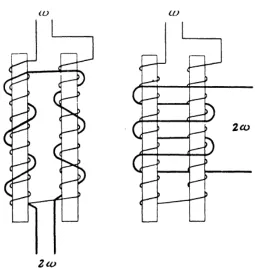
instrument to infer these quantities. Figure 2-1 shows the basic configuration of two versions of a

rodcore design, in which two sets of windings encircle the permeable material. The inner winding

(marked ω) is known as the drive or excitation winding, and is used to cyclically saturate the

magnetic core in opposite directions by passing a known alternating current through the wire.

The outer winding (marked2ω) is the sense or pick-up winding which will produce a voltage that

depends on the magnetic flux it detects within the core.

2.2.1 Mechanical Design

While a single rod-core design is the simplest magnetometer construction, having dual cores allows

the drive signal to be masked from the sense winding through a phase shift between the two

cores. Since the Apollo 16 mission, however, space science missions have focused on the ring core

magnetometer design [Dyal et al., 1973]. This design makes use of the field generated by the drive

coils acting in opposite directions for each half of the sensor, similar to the operation with two rod

cores as shown in Figure 2-1. For a ring-core design, the permeable material forms a ring shape,

often wound as a thin tape onto a non-magnetic bobbin. The drive coil is then wound toroidally

(36)

Figure 2-1: Cartoon showing two versions of the basic rod-core magnetometer sensor design fromDolginov et al.[1961]

Figure 2-2: Cartoon showing the construction of a ring-core magnetometer design from

(37)

In Figure 2-2 we can see a cross-sectional cartoon of a ring core instrument taken from Dyal

et al.[1973]. The inner core material is made up of multiple windings of a magnetically permeable

tape, and is wrapped by the drive coil. The sense coil covers this whole structure, which is in

turn covered by a feedback winding. In order to increase the linearity of the performance of the

instrument, this feedback winding is sometimes used to maintain the field measured by the sense

coil at nullity, and the actual output measurement is determined by the voltage applied to the

feedback winding to maintain this value coupled with the sensor output. The sense and feedback

coils can be combined into a single wrap though careful signal separation within the electronics.

The racetrack design elongates this core into an exaggerated oval, providing more material

aligned with the sense axis to respond to the background field component in the axial direction. This

operation works similarly to the rod core design, but dispenses with the dipolar field components

emanating from the ends of the rods. These extraneous field components, often referred to as fringe

magnetic fields, contribute non-aligned components of the field to the measurement and generally

disrupt the otherwise magnetically clean environment. For the following discussion of this work,

we will focus on the ring core design which includes the racetrack geometry.

2.2.1.1 Core Material

For the material used to make up the core, the most desirable trait is its high magnetic permeability.

There are additional constraints given the environment in which the instrument will be used, such

as expansion coefficients and the effect of temperature on the permeability. For the use of a fluxgate

both on the ground and in the space environment, the best material found to date is known as the

6-81 permalloy [Gordon et al., 1968]. The chemical mixture of this material is 6% Molybdenum,

81.3% Nickel, and 12.7% Iron.

A property of any ferromagnetic material is the closed hysteresis loop (see Figure 2-3). This

(38)

Figure 2-3: Depiction of standardized hysteresis curve fromGubbels [2017] (courtesy ofIndustrial Heating). Points 1, 2, and 3 show transition to uni-form magnetic field orientation B in material due to externally applied field H. Inset shows stepwise jumps known as Barhausen Noise (BN) typical in ferromagnetic materials.

field. The loop implies that this is not a single-valued function, but that the material retains a

memory of its magnetization. Once the external field is reduced to nullity after the material is

saturated in a particular direction, the material will remain somewhat magnetized in this same

direction (the degree of remnant magnetization is unique to each material). A nonzero external

field applied in the reverse direction is necessary to reduce the material magnetization to zero. The

reverse of this process then occurs as the material is brought into opposite saturation and back

again to zero through a cyclically applied external field.

The cause of this magnetization dependence can be traced to the magnetic domains within the

material. Any crystalline structure that is not composed of a single uniform crystal lattice will be

made up of multiple crystallites, also known as grains. These grains are uniform in their internal

crystal lattice structure, but are misaligned with each other, creating distinct boundaries at the

interface between grains. Grain orientations are spontaneous and randomly directed as the lattices

join together, and the volume attributed to grain boundaries (proportional to the surface area of

(39)

The crystallite grain is further divided into several magnetic domains, each comprised of

ho-mogeneously aligned dipolar structures. These domains will preferentially be aligned parallel to

the “easy” magnetization direction of the grain, and form spontaneously when the material falls

below the Curie temperature. For the lowest expenditure of energy, they will be evenly divided into

domains aligned parallel and anti-parallel with the easy magnetization direction. The widths of the

domains are inversely proportional to the thickness of the grain boundary [Carey and Isaac, 1965],

leading to a decrease in the overall extent of the domain wall and the stored potential magnetization

energy therein. This in turn means the internal magnetization energy is reduced for thinner grain

boundary widths.

The main source of noise in a fluxgate magnetometer due to the permeable core material is due

to so-called Barkhausen noise. This can be seen in the inset of Figure 2-3, where rather than a

smooth transition along the hysteresis curve, the path will be made up of small stepwise jumps. Due

to the random orientation of crystal grains, these jumps are unpredictable and unlikely to repeat

upon subsequent cyclic remagnetizations of the material. As such, this will result in an uneven

measurement of the external dc field which forms the ultimate noise floor of the instrument.

The reason for these jumps is related to the release of magnetization energy during the

re-orientation of magnetic domains, and it is believed that this energy release is increased at grain

boundaries. This source is still not fully understood, but some researchers [Narod, 2014, e.g.] have

proposed a model of domain reversals based on reorientation of “channel domains” during

satura-tion by means of magnetic reconnecsatura-tion. These channel domains convert to and from the typical

“stripe domains” observed byAmos et al.[2008] using magnetostatic energy, which is concentrated

at grain boundaries due to the mismatched preferred magnetic field orientations. Grain boundaries

are reduced in thickness and in number by increasing the sizes of the grains themselves, which can

(40)

to increase the grain size of the permalloy material used in the racetrack magnetometer by extending

the annealing time at temperatures conducive to grain growth, as described in section 2.3.1.1.

2.2.1.2 Sense/Drive Coil Operation

The drive winding, wound uniformly along the length of the core material is stimulated with an

alternating current which cyclically drives the core into alternate magnetic saturation. In our case,

this winding is toroidal in shape, generating alternating fields that are cyclically aligned clockwise

followed by counter-clockwise. The current is most often applied with a square wave, but can also

be applied with a simple sinusoid.

The important aspect is that the core material reaches saturation such that the permeability

falls away to that in a vacuum. At this point, the magnetic resistance in the core rapidly increases

and the magnetic flux through the sense coil collapses. Once the applied voltage reverses, the core

recovers from saturation and the changing magnetic flux is once again detected by the sense coil.

Since the entirety of the ring core is surrounded by the sense winding, this changing magnetic flux

measurement is canceled out.

In the case of the existence of an external field, we can think of the permeable core as being

comprised of two half-cores symmetric about the helical axis of the sense winding. The component

of the field along this axis will permeate the core, and so will contribute to the induced toroidal

field of one half towards saturation, and detract from the other. Uneven saturation of the core

material will result in the effective decreased permeability of the counter-aligned half of the core.

Until reaching this point of partial saturation, the total field induced within the core along the

sense axis adds to zero. Once partial saturation is reached, however, the sense coil encompasses

an axial flux in the magnetic field that changes with the increasing drive current until both halves

are fully saturated. The changing magnetic flux during the period of partial saturation induces an

(41)

Figure 2-4: Analytical applied and sensed waveform derivations for a fluxgate magnetometer fromGordon and Brown[1972]© IEEE.

The emf induced in the sense winding by the changing flux will peak in an alternating positive

and negative direction on either side of the change in applied drive voltage (see Figure 2-4), resulting

in an output signal at twice the frequency of the drive signal. The magnitude of the field component

along this axis is given by the amplitude of this output signal, and the phase of the signal will provide

the sense of the field along this axis.

2.3 Racetrack

The fluxgate magnetometer has been an integral piece of hardware to most space-science missions

since the beginning of the space age. A DC measurement of the field is often necessary to determine

local plasma parameters as well as for relative positioning and orientation for any other on-board

measurements, while AC changes are necessary for wave and field gradient studies. As research

questions become more specific and refined, the measurement apparatus used to answer these

questions must also improve. Our efforts to develop a low-noise magnetometer for these purposes

are rooted in the optimization of a “racetrack” based design with a concentration on improving the

(42)

2.3.1 Material Development

While these instruments have been in use for many years, there has been little advancement into

their capabilities, and the 6-81 permalloy material with which many are made comes from a finite

and dwindling supply [Acuña, 2002]. We have acquired supplies matching the correct composition

ratios as the Infinetics 6-81 permalloy, and have experimented with the annealing process to improve

the permeability performance.

2.3.1.1 Crystal Structure

As described in section 2.2.1.1, the most basic source of noise in a fluxgate magnetometer

irre-spective of electronic advances is within the permeable material itself. In order to minimize the

magnetostatic energy contained within grain boundaries that leads to Barkhausen noise during

do-main flips, we have introduced a process to increase the growth of crystallite grains, thus reducing

the surface area of intergrain boundaries.

Samples of the permeable material already rolled to 100 µm thick ribbons and slit to the

speci-fications needed for the fluxgate sensor construction were set aside and coated with an electrically

insulating magnesium hydroxide solution. These were then subjected to a heat treatment

proce-dure adapted from that described by Gordon et al. [1968]. Starting from room temperature and

confined within a furnace to an atmosphere consisting of 95% Ar and 5% H, the first sample was

immediately brought up to the annealing temperature of 1050◦C. The sample was held at that

temperature for 20 hours with consistent positive air pressure from the furnace chamber leading

through an exhaust tube submerged in water. Care was taken to ensure oxygen did not enter the

chamber during the heating process. At this point the second sample was added to the furnace,

and both were held at 1050◦C for a further 4 hours.

After this sustained bake, the samples were allowed to cool at their natural rate to 600◦C. The

(43)

Figure 2-5: Electron microscope images of the Permalloy material after two different heat treatment processes. The left (right) image shows the visible grain structure of the alloy after an annealing process during which it is held at 1200◦C for 4 (24) hours.

a controlled rate of 36.6◦C/hr until they reached 250◦C. This temperature range is the so-called

“critical ordering range” [Gordon et al., 1968] surrounding the material Curie point of _∼460◦C

[McLyman, 2004], and is where we expect to see crystallite grain growth and magnetic domain

formation. Enoch and Fudge [1966] demonstrate that the peak permeability for a molybdenum

alloy composed of 80.9% Ni, 13.1% Fe, and 6% Mo is achieved at a cooling rate between 30-40

◦_{C/hr, which we targeted with the 36.6}◦_{C/hr rate. The samples were allowed to further cool to}

room temperature at the natural exothermic rate.

We examined the samples from these two batches, one which was held for 24 hours and the other

for 4 hours at 1050◦C followed by simultaneous cooling processes, under an electron microscope to

determine any effects on grain size. The results can be see in Figure 2-5, where the 4-hour sample

can be seen on the left, and the 24-hour sample on the right. There is a clear in crease in grain

sizes from the 4-hour to the 24-hour sample. Additionally, the grain boundaries are much less

(44)

2.3.2 Geometry

As we mentioned in section 2.2.1, a racetrack design is based on the same concept as the ring core

magnetometer, but involves elongating the ring shape along one axis. The purpose of this design

is to increase the amount of permeable material aligned with the desired measurement direction,

and maintain a linear measurement axis contained by the sense winding to minimize cross-field

noise. An example diagram can be see in Figure 2-6 where the toroidal drive coil given by nprim is

wound around several wraps of permeable tape. The sense coil (shown as nsec) is shown covering

the whole device, such that the sense axis normal to the coil cross-section is aligned with the long

straight portions of the permeable tape.

2.3.2.1 Optimization

Previous studies have demonstrated the viability and noise profiles of various configurations of

a fluxgate sensor [Hinnrichs et al., 2001], but have limited these observations to the laboratory

environment. Our experiments thus far with altering the geometry of the instrument have proven

very successful. By extending the sensor into a racetrack configuration rather than the typical

circular shape (see lcore in Figure 2-6), we are able to extend the axis along which a measurement

is made and reduce the influence from fields operating in perpendicular directions.

By concentrating our measurements along a particular axis, we are able to increase the

sensi-tivity of our sensor at the expense of an increased size both of each sensor and of the instrument

as a whole. The circular ring cores have the advantage of being able to sample an external field in

two axes simultaneously, cutting down on the number of cores needed. One also has the ability to

rotate the core within the frame holding the sense winding in order to balance out any aberrative

measurements due to asymmetry of construction.

Nevertheless, we believe that the increased sensitivity gained from the axial optimization

In Situ Observations of Pearl Pulsations and Development of a Low-Noise Fluxgate Magnetometer, Kristoff Paulson

University of New Hampshire

University of New Hampshire Scholars' Repository

Doctoral Dissertations

Student Scholarship

Winter 2018

In Situ Observations of Pearl Pulsations and

Development of a Low-Noise Fluxgate

Magnetometer

Kristoff Paulson

Follow this and additional works at:

https://scholars.unh.edu/dissertation

Recommended Citation

In situ observations of pearl pulsations and

development of a low-noise fluxgate magnetometer

KRISTOFF PAULSON

Acknowledgments

Table of Contents

List of Tables

List of Figures

ABSTRACT

Chapter 1

Introduction

1.1

What is a Space Plasma?

1.2

Plasma Waves

1.3 Particle Motion

1.4

Magnetosphere

1.5

Solar Wind as a Driver

Chapter 2

Magnetometer Design

2.1

Applications

2.2 Traditional Fluxgate

2.3

Racetrack