Data MiningAssociation Rules

Data MiningAssociation Rules

University of Nicosia, 46 Makedonitissas Avenue, P.O. Box 24005, 1700 Nicosia, Cyprus [email protected], [email protected], [email protected]

Abstract -Business Intelligence (BI) refers to a broad category of applications which assist executive business users to improve their decisionmaking and strategic planning by collecting, storing and analysing a large volume of historically collected data. BI systems may be divided into reporting systems and data mining applications. Data mining (also known as Knowledge Discovery in Data, or KDD) is the science of extracting useful knowledge from huge data repositories. Data Mining applications often employ sophisticated mathematical and statistical techniques to perform data analysis, search for specific patterns or relationships, if they exist, and make future predictions.

This paper focuses on link analysis used by Data Mining systems to extract associations between individual data records or data sets involved in the same event. It demonstrates an implementation of the SETM algorithm with custom modifications made to expand functionality and improve time and space complexity. The system makes use of the frequent itemsets to generate association rules, while also calculating supportand confidence. The algorithms are integrated in a user-friendly system which can be used to generate frequent itemsets and extract association rules online in real time.

Keywords: Business Intelligence, Data Mining, SETM algorithm.

I. INTRODUCTION

A. What is Business Intelligence?

Business Intelligence refers to a broad category of applications and technologies which serve the purpose of collecting, storing, analysing and providing access to data with the purpose of helping business users to make better business decisions [1]. Business data can be any type of data related to a business or organization but is usually sales data, transaction history, customer records, employee records or any kind of stored data which can be analyzed (usually statistically or mathematically)[2]. Such data is stored in computerized databases or larger data repositories such as data warehouses. After the business data is analyzed by a business intelligence system, new information can be obtained or existing but hidden information is revealed.

BI can also be described as the business process which involves a series of activities used to gather and analyze data and distribute the results to those requiring them in order to improve decision-making [3].

B. The role of Business Intelligence in an organisation BI is extremely vital to organisations and their employees since they need access to timely information and analysis of that information [4].

In order to pursue more strategic BI, organisations must be able to effectively manage all the data at their disposal. The

information that is retrieved must be of very high quality standards. If not, then this effectively means that organisations will be limited to a less strategic BI approach. To be successful in its data analysis a business must possess fast, relatively cheap data warehouses required to effectively support BI [4].

A data warehouse refers to a database system that includes data, programs, and the necessary personnel who specialise in the preparation of data for BI processing.Fig. 1below illustrates the components of a data warehouse [5]. Data are read from operational databases by the Extract, Transform and Load (ETL) System.This system will clean and prepare the data in order to be processed for BI. The extracted data will be stored in a data warehouse using a data warehouse Database Management System (DBMS). Additionally, metadata concerning the data’s source, format assumptions, etc., is maintained. The data warehouse DBMS will then extract data and forward them to BI Tools with which BIusers interact [5].

Fig. 1. Data Warehouse Components (Revised – Kroenke and Auer, [5])

BI systems are also referred to as Decision Support Systems since they assist organisations with their decision making [5]. They are used in analysing present and past activities of the organisation but also in accurately predicting future events. BI systems do not support operational activities such as processing or recording of orders. Instead, they support managers in their planning, analysis, control, and decision- making tasks.

Fig. 2. The role of Business Intelligence Systems in decision making (Revised from Olszak and Ziemba [2])

BI systems should make it possible for the users to set precise objectives and to execute these objectives. Furthermore, they provide a basis for decision making and allow the optimisation of future actions by acting upon various aspects of the company’s performance. Ultimately, they help enterprises to realise their strategic objectives more effectively [2].

To summarize, BI technologies provide historical, current and predictive views of business operations. Common functions of business intelligence technologies are reporting, online analytical processing, analytics, data mining, process mining, complex event processing, business performance management, benchmarking, text mining and predictive analytics.

C. Data Mining

Data mining (also known as Knowledge Discovery in Data, or KDD) is the science of extracting useful knowledge from huge data repositories [6]. More specifically this useful knowledge usually refers to hidden and unexpected patterns and relationships in sets of data [7]. Data mining applications use mathematical and statistical techniques to perform what-if analysis, discover new patterns, make future predictions, and therefore assist in decision making. Their central activity being “discovery” aims at identifying specific patterns or relationships met frequently or classified as unusual. An unusual pattern for example could relate to credit card usage. If the card owner does not normally use his/her credit card much, a very rapid increase in usage could possibly mean that the card was stolen. Such an application could very likely help detect credit card fraud by monitoring credit card usage for each owner [8].

Data Mining Operations and Techniques

Table I below presents and briefly describes the four main operations supported by Data Mining applications and the techniques associated with them.

TABLE I

DATA MINING OPERATIONS AND TECHNIQUES (EXTRACTED FROM [7])

Operations Data Mining Techniques

Predictive modelling: Analyzes data to determine essential characteristics (model).

Classification: Establishes a specific predetermined class for each data record.

Value prediction: Estimates a

continuous numeric value

associated with each data record. Database segmentation:

Partitions a database into a number of homogeneous segments.

Demographic or Neural clustering: Establish allowable data inputs to be used for analysis by calculating the distance between records. Link analysis:

Establishes links, called associations, between records or sets of them in a database.

Association discovery: Finds items that imply the presence of other items in the same event. Sequential pattern discovery: Finds patterns between events. Similar time sequence discovery: Finds links between two sets of data that are time-dependent.

Deviation detection: Identifies outliers.

Statistics: Identify outliers using for example linear regression.

Visualization: Displays summaries and graphs to make deviations easy to detect.

II. ASSOCIATION RULES

An association rule is a rule which implies certain association relationships among a set of objects, such as “occur together” or “one implies the other”, in a database[9]. They were intensively studied [10, 11, 12]. See [13, 14] for some detailed surveys.

Let I = {i1, i2, …, im} be a set of literals called items. The

database consists of a set of sales transactions T [15]. Each transaction T is a set of items such that T⊆I. A transaction T is said to contain the set of items X if and only if X⊆ T.

An association rule is an expression of the form X→Y, where X⊆I and Y⊆I are sets of items [16]. The intuitive meaning of such a rule is that the presence of the set of items X in a transaction set also indicates a possibility of the presence of the itemset Y. In plain English this means that the transactions of the database which contain X tend to contain Y as well.

III. ASSOCIATION ALGORITHMS

The Apriori Algorithm

Probably the most famous of all association rule mining algorithms, Apriori has been developed for rule mining in large transaction databases by IBM's Quest project team [18, 19]. They have decomposed the problem of mining association rules into two parts:

• Find all combinations of items that have transaction support above minimum support. Call these combinations frequent itemsets.

• Use the frequent itemsets to generate the desired rules. The general idea is that if, say, ABCD and AB are frequent itemsets, then we can determine if the rule ABCD holds by computing the ratio r= support(ABCD)/support(AB). The rule holds only if r >= minimum confidence. Note that the rule will have minimum support because ABCD is frequent.

The Apriori algorithm in pseudo code appears in Fig. 3.

L1 = {large 1-itemsets};

for ( k = 2; Lk-1 ≠∅; k ++) do begin Ck = apriori-gen(Lk-1); // New candidates

forall transactions t ∈ D do begin

Ct = subset(Ck, t); // Candidates contained in t

forall candidates c ∈ Ctdo

c.count++;

end

Lk = {c ∈ Ck | c.count ≥ minsup};

end

Answer = ∪kLk;

Fig. 3. The Apriori algorithm in pseudo code [19]

Apriori makes multiple passes over the database. In the first pass, the algorithm simply counts item occurrences to determine the frequent 1-itemsets (itemsets with 1 item). A subsequent pass, say pass k, consists of two phases. First, the frequent itemsets Lk-1 (the set of all frequent (k-1)itemsets)

found in the (k-1)th pass are used to generate the candidate itemsets Ck (that is candidates to become frequent itemsets)

using the apriori-gen() function.

This function first joins Lk-1 with Lk-1, the joining condition

being that the lexicographically ordered first k-2 items are the same. Next, it deletes all those itemsets from the joined result that have some (k-1)-subset that is not in Lk-1 yielding Ck. The

algorithm then scans the database.

For each transaction, it determines which of the candidates in Ck are contained in the transaction using a hash-tree data

structure and increments the count of those candidates. At the end of the pass, Ck is examined to determine which

candidates are frequent, yielding Lk. The algorithm terminates

when Lk becomes empty.

The SETM Algorithm

The SETM algorithm was motivated by the desire to use SQL to compute large itemsets [20, 21]. Ck (Lk) represents the

set of candidate itemsets in which the Transaction Identity (TID) of the generating transactions has been associated with the itemsets. Each member of these sets is of the form < TID, itemset>. The TID uniquely identifies each transaction, much like a primary key in a database table.

In SETM algorithm candidate itemsets are generated on the fly as the database is scanned. After reading a transaction, it is determined which of the itemsets that were found to be frequent in the previous pass are contained in this transaction. New candidate itemsets are generated by extending these frequent itemsets with other items in the transaction. A frequent itemset L is extended with only those items that are frequent and occur later in the lexicographic ordering of items than any of the items in L.

The candidates generated from a transaction are added to the set of candidate itemsets maintained for the pass. In order to use the standard SQL join operation for candidate generation, SETM separates candidate generation from counting. It saves a copy of the candidate itemset together with the TID of the generating transaction in a sequential structure (such as a temporary table).

At the end of the pass, the support count of candidate itemsets is determined by sorting and aggregating this sequential structure.

SETM remembers the TIDs of the generating transactions with the candidate itemsets. To avoid the need of a subset operation, it uses this information to determine the frequent itemsets contained in the transaction read.

The final relation Ck is obtained by deleting those

candidates that do not have minimum support. Assuming that the database is sorted in TID order, SETM can easily find the frequent itemsets contained in a transaction in the next pass by sorting the data by TID. In fact, it needs to visit every member of Ck only once in the TID order, and the candidate

generation can be performed using the relational merge-join operation.

The algorithm consists of a single loop, in which two sort operations and one merge-scan join are performed. The first sort is needed to implement the merge-scan join that follows it. The second sort is used in order to generate the support counts efficiently. Generating the counts involves a simple sequential scan over the Rk relation.

In Fig. 4 below the algorithm is presented in pseudo code. k =1;

sort R1 on item;

C1= generate counts from R1;

repeat

k = k+1;

sort Rk-1 on trans_id, item1,…itemk;

Ck = generate counts from Rk′;

Rk = filter Rk′to retain supported patterns;

until Rk=∅;

Fig. 4 The SETM algorithm in pseudo code

IV. AIMS AND OBJECTIVES OF THE STUDY

This paper focuses on link analysis used by Data Mining systems to extract associations between individual data records or data sets involved in the same event. It demonstrates an implementation of the SETM algorithm with custom modifications made to expand functionality and improve time and space complexity. The system makes use of the frequent itemsets to generate association rules, while also calculating support and confidence. The algorithms are integrated in a user-friendly system which can be used to generate frequent itemsets and extract association rules online in real time.

The implementation aspect of this project aims to solve the problem of a computerized, fully working solution for a data mining system that produces association rules. The system allows a user to select attributes of a database along with the frequency, support and confidence of a rule. It then scans the database and generates frequent itemsets for the user’s selections. Finally, it produces association rules for the aforementioned selections.

V. THE DATABASE

The case uses a real medical database with historical patient data which includes blood analysis results, blood pressure measurements, clinical history data, and other. The patients described are people who have sustained or are in danger of sustaining a stroke.The data was prepared for use by completing the following activities:

• The data was cleaned by removing missing or incomplete values.

• Numerical values were changed to characters.

• The layout of the database was changed from a horizontal to a vertical layout.In the horizontal layout, all the attributes are in columns whereas, in the vertical layout all the attributes are seen as transactions, so there are only two columns; the first column is the Patient Id and the second is a valued attribute of the patient e.g. Cholesterol.

• The original database was in the form of a spreadsheet file which was then converted to a database.

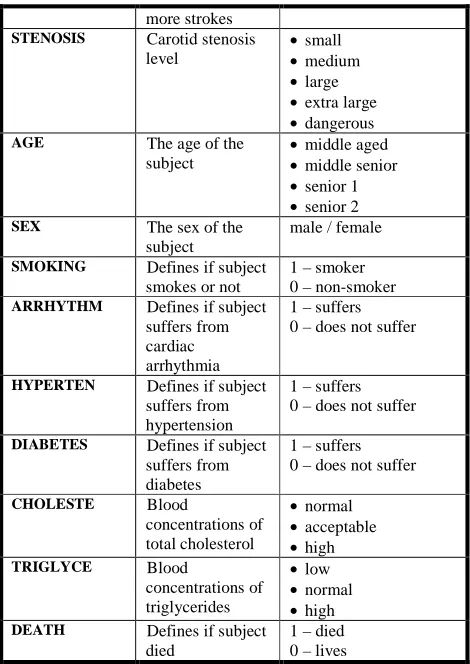
A data dictionary presenting the contents of the database is shown in Table II below.

TABLE II

DATA DICTIONARY OF THE MEDICAL DATABASE

Attribute Attribute description

Unit of measurement

ID The unique

identifying number of each subject

-

IEVENT Defines if subject suffered one or

1- suffered 2- didn’t suffer

more strokes STENOSIS Carotid stenosis

level

•small

•medium

•large •extra large •dangerous

AGE The age of the

subject

•middle aged •middle senior •senior 1 •senior 2

SEX The sex of the

subject

male / female

SMOKING Defines if subject smokes or not

1 – smoker 0 – non-smoker ARRHYTHM Defines if subject

suffers from cardiac arrhythmia

1 – suffers 0 – does not suffer

HYPERTEN Defines if subject suffers from hypertension

1 – suffers 0 – does not suffer

DIABETES Defines if subject suffers from diabetes

1 – suffers 0 – does not suffer

CHOLESTE Blood

concentrations of total cholesterol

•normal •acceptable •high TRIGLYCE Blood

concentrations of triglycerides

•low •normal •high DEATH Defines if subject

died

1 – died 0 – lives

A statistical analysis of the database was performed before this was converted from horizontal to vertical. The results appear in Table III (inserted at the end of the paper).

VI. ASSOCIATION ALGORITHM USED

For the implementation described in this paper the SETM algorithm was selected mainly because this can be implemented in pure SQL and uses only simple database primitives, namely sorting and merge-scan join. Moreover, the SETM algorithm is simple, flexible, fast, and scales very well. However, since for the purpose of this study, we are interested in calculating frequent k-itemsets with specific elements, the following modifications to the generic SETM algorithm were considered appropriate (modifications are described in SQL code as well):

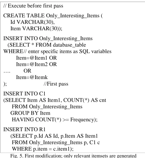
1) First modification: Generation of frequent itemsets with specific items

a greatly reduced data set while at the same time reducing the chance of overfilling the RAM of the PC, and thus using the hard disk for saving the intermediate results. Subsequently, the algorithm will now execute in only a fraction of the time and will use minimal memory resources. The final results will still be correct as items 1-10 will be included in the association rules.

Fig. 5 below shows the first modification made to the algorithm.

// Execute before first pass

CREATE TABLE Only_Interesting_Items ( Id VARCHAR(30),

Item VARCHAR(30));

INSERT INTO Only_Interesting_Items (SELECT * FROM database_table

WHERE // enter specific items as SQL variables Item=@Item1 OR

Item=@Item2 OR

…. OR

Item=@Itemk

); //First pass

INSERT INTO C1

(SELECT Item AS Item1, COUNT(*) AS cnt FROM Only_Interesting_Items

GROUP BY Item

HAVING COUNT(*) >= Frequency);

INSERT INTO R1

(SELECT p.Id AS Id, p.Item AS Item1 FROM Only_Interesting_Items p, C1 c WHERE p.item = c.item1);

Fig. 5. First modification; only relevant itemsets are generated

2) Second modification: Generation of an association rule and calculation of support and confidence

The algorithm can be further expanded so that after it has generated all the related frequent itemsets it can use them to calculate an association rule for them. This can be done in the following steps:

At first, the structure of the association rule needs to be defined.Then, the support and the confidence of the rule need to be calculated. Remember that for the rule A→B we have:

Support (A→B) = Probability (A∪B) = ୡ୭୳୬୲(୅∪୆)

ୡ୭୳୬୲(୲୭୲ୟ୪)

Confidence (A→B) = Probability (B|A) = ୡ୭୳୬୲(୅∪୆)

ୡ୭୳୬୲(୅)

The support and confidence for an association rule for any frequent k-itemset can therefore be calculated in SQL as follows in Fig. 6.

// Support

SET @Support = (SELECT cnt FROM Ck WHERE

(Item1 = @Dimension1 OR Item1 = @Dimension2 OR … Item1 = @Dimensionk OR Item1=@Measure) AND (Item2=@Dimension1 OR Item2 = @Dimension2 ... OR item2 = Dimensionk OR Item2=@Measure)

…

AND (Itemk=@Dimension1 OR Itemk = Dimension2 OR ... Itemk = Dimensionk OR Itemk=@Measure) )/Total_Items_In_Database;

// Confidence

SET @Confidence = @Support / ( (Select cnt from Ck-1

WHERE

(Item1 = @Dimension1 OR Item1 = @Dimension2 … OR Item1 = @Dimensionk) AND

(Item2 = @Dimension1 OR Item2 = @Dimension2 … OR Item2 = @Dimensionk) AND

…

(Itemk-1 = @Dimension1 OR Itemk-1 = @Dimension2 … OR Itemk-1 = @Dimensionk)

) / Total_Items_In_Database );

Fig. 6. Second modification; Calculating Support and Confidence

The algorithm was expanded to store the results, along with the support and confidence,in a results table after checking if the produced ruleis a strong rule, i.e., it satisfies minimum support and confidence (see Fig. 7).

CREATE TABLE ANSWER (Message VARCHAR (200)); IF @Support >= @Min_support/100.0 AND

@Confidence >= @Min_confidence/100.0 BEGIN

INSERT INTO ANSWER

(SELECT 'The selected items generate this rule:') INSERT INTO ANSWER

(SELECT @Dimension1+' AND '+@Dimensionk+ ' => ' +@Measure)

INSERT INTO ANSWER

(SELECT 'With Support= '+(CONVERT (VARCHAR(5), @Support)) +' and Confidence= '+(CONVERT

(VARCHAR(5), @Confidence))) END

ELSE BEGIN

INSERT INTO ANSWER

(SELECT 'Items selected do not satisfy min support or confidence so no rules are generated')

SELECT * FROM ANSWER DROP TABLE ANSWER END

GO

Fig. 7. Second modification; Generation of rules

3) Third modification: Generation of multiple association rules

generating the confidence and support for each individual member in each itemset with its generation. This means that support, confidence and association rules, are all calculated at each pass of the algorithm for each member of the itemset. For example, at the second pass, support, confidence and association rules will be calculated for all members of the 2-itemset.

Furthermore, the input parameters of each stored procedure were modified to allow a wildcard search for each item. The original database had to be re-categorized to allow for a unique wildcard search for each category.

The above translate to the SQL script shown in Fig. 8.

// Execute at the end of each pass of the algorithm

SELECT b.Item_x+' => '+b.Item_y+' With Support= ' + CONVERT(VARCHAR(500), CAST ( (b.cnt*100.0) /@Subjects_No AS NUMERIC(5,2))) +'%

AND Confidence= ' ++ CONVERT(VARCHAR(500), CAST ( (b.cnt*100.0) / a.cnt AS NUMERIC(5,2))) +'%' FROM table_x-1 a , table_x b

WHERE a.Item_x=b.Item_x

GROUP BY a.cnt, b.cnt, b.Item_x,b.Item_y HAVING b.cnt >= 0

AND b.cnt/(@Subjects_No/100.0) >= @Min_support AND (b.cnt*1.0) / (a.cnt/100.0) >= @Min_confidence;

Fig.8. Third modification: Support and confidence for multiple rules

4) Fourth modification: Making the order of the items in itemsets important

Originally, the algorithm was designed to generate all itemsets in a lexicographical manner. This means that it creates unique itemsets by taking unique combinations of items. It also means that the order of the items in an itemset is not considered important, i.e., the itemset {Stroke, Male} would be considered the same as the itemset {Male, Stroke}. In this case, only one of the aforementioned itemsets would be generated. Assuming though that both itemsets were available, the resulting association rules from these two itemsets would be:

Male=>Stroke Support: x%, Confidence: y% Stroke=>Male Support: x%, Confidence: y%

These rules have totally different meanings:The first states the probability to have a stroke if you are male while the second shows from the total people who had a stroke, what percentage is male. It is therefore important to obtain all the rules. This can be easily done by a simple inequality test for both items at the time of their generation (see Fig. 9.).

INSERT INTO RTMPk

(SELECT p.Id AS Id, p.Item1 AS Item1, p.Item2 AS Item2, …, p.Itemk-1 AS Itemk-1, q.Itemk-1 AS Itemk FROM Rk-1 p, Rk-1 q,

WHERE p.Id = q.Id AND p.Item1 = q.Item1 ... AND p.Itemk-2 = q.Itemk-2

// The following line has to be replaced by the line below

AND p.Itemk-1 < q.Itemk-1;

AND p.Itemk-1 <> q.Itemk-1;

Fig. 9. Fourth modification: Making the order of the items in an itemset important

VII. IMPLEMENTATION AND SAMPLE RESULTS

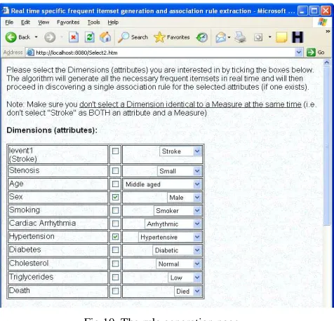
The modified SETM algorithm was implemented and a user-friendly environment was created whereby the user beginsby selecting a number of dimensions to run the association algorithm, by ticking checkboxes and selecting from the drop down menus (see Fig. 10).

Fig.10. The rule generation page

After the dimension selection the user can enter the desired frequency, support and confidence of the generated association rules.

Fig.11. Association rule for dimension selection

The SETM algorithm has been tested on the database for a number of x-itemsets (where x represents an integer from 1 to 11 itemsets). For more clarity, a 3-itemset for example, will consist of sets of items with exactly 3 members in each set. After all the itemsets are found, a mathematical function is applied to find frequent itemsets, i.e., only those itemsets that satisfy a minimum support and confidence. An association rule is extracted by taking the generated frequent itemsets and the user-supplied support and confidence into account. The rule will depend upon the user attribute selection(s). For example, the user could select the attributes “cholesterol” and “hypertension” as dimensions and “stroke” as measure, to find an association rule (if one exists) for the relationship between cholesterol and hypertension as the cause of stroke.

VIII. SUMMARY AND CONCLUSIONS

This paper presented an implementation of the SETM algorithm in a medical data mining application. The algorithm has undergone some customization to expand its functionality and improve time and space complexity. It was then tested on the database for a number of x-itemsets. Association rules were extracted successfully, support and confidence were calculated. The implementation also demonstrated how tight coupling between a DBMS and a Data Mining system can be fully achieved.

IX. FUTURE WORK

Since the implementation presented in this paper involved a real medical database, the results regarding the association rules extracted by the data mining application, could be cross-checked against statistically-proved results reported in the medical profession. By performing this exercise one could establish two things: 1) the credibility of the medical database used, even though this originated from the records of a single

doctor, and 2) the credibility of the data mining application and the modified algorithm.

A future addition to the online real-time data mining application can be the provision for uploading / importing new data.

In terms of the modified / customized SETM algorithm, this needs to undergo benchmark tests in order to establish the originallyintended improvements in time and space complexity.

REFERENCES AND BIBLIOGRAPHY

[1] L. Rossetti,“What is business intelligence (BI)?,” http://searchdatamanagement.techtarget.com/definition/b usiness-intelligence,2006. (Last accessed October 2011) [2] C. M. Olszak, E. Ziemba, “Approach to building and

implementing Business Intelligence

Systems”,Interdisciplinary Journal of Information, Knowledge, and Management, Vol. 2, pp. 135-148, 2007.

http://ijikm.org/Volume2/IJIKMv2p135-148Olszak184.pdf (Last accessed November 2011) [3] S. Misner, Microsoft Corp., “Business Intelligence:

planning your first BI solution”,

http://technet.microsoft.com/en-us/magazine/gg413261.aspx., 2009. (Last accessed October 2011)

[4] M. Smith., “BI is serious business”,

http://businessintelligence.com/research/302, 2010. (Last accessed October 2011)

[5] D.M. Kroenke, and D.J. Auer,Database Processing: Fundamentals, Design, and Implementation, 11th Intern. Ed., NJ, Pearson Education (US), 2009, pp. 134-136, 162-163, 556-571, 584-585.

[6] ACMSIGKDD,“Data Mining curriculum", http://www.sigkdd.org/curriculum.php, 2006. (Last accessed November 2011)

[7] T. M. Connonly, C. E. Begg, Database Systems: a Practical Approach to Design, Implementation, and Management, 5th_{Ed, Addison-Wesley, 2010.}

[8] R.A. Elmasri, and S.B. Navathe,Database Systems: Models, Languages, Design, and Application Programming”, 6th Global Ed., NJ, Pearson Education (US), 2010, pp. 3-4, 23, 309.

[9] De Alwis, A. S. Malinga, K. Pradeeban, W. A. Weerasiri, “Association rule mining with extended vertical format data mining”, Department of Computer Science and Engineering, University of Moratuwa, Sri Lanka, 2009. [10]A. Savasere, E. Omiecinski, S. Navathe, “Mining for

customer transactions”, Proc. of ICDE, pp. 494-502, 1998.

[11]J. Han, J. Pei, and Y. Yin,“Mining frequent patterns without candidate generation”, Proc. of the 2000 ACM SIGMOD Intern. Conf. on Management of Data, USA, 2000.

[12]S. Brin, R. Motwani, C. Silverstein, “Beyond market baskets: generalizing association rules to correlations”, Proc. of ACM SIGMOD Conf., pp. 265-276, 1997. [13]J. Hipp, U. Guntzer, G. Nakhaeizadeh, “Algorithms for

association rule mining – a general survey and comparison”, SIGKDD Explorations, Vol. 2(1), pp. 58-64, 2000.

[14]S. Kosiantis, D. Kanellopoulos, “Association rules mining: a recent overview”, GESTS Intern. Transactions on Computer Science and Engineering, Vol. 32(1), pp. 71-82, 2006.

[15]K. Rajamanim, A.Cox,“Efficient mining for association rules with relational database systems”, Proc. of the 1999 Intern. Symposium on Database Engineering & Applications, pp. 148.

[16]Karuna Pande Joshi, “Analysis of Data Mining algorithms”, TechReport, UMBC, March 1997.

[17]R. Agrawal, T.Imielinski, A.Swami, “Mining association rules between sets of items in large databases”, Proc. ACM SIGMOD Conf. Management of Data, pp. 207-216, May 1993.

[18]L. Wei,A. Mozes, “Computing frequent itemsets inside

Oracle 10G”, VLDB, Toronto, Canada, August 2004, pp.

1253-1256.

[19]R. Agrawal, R. Srikant, “Fast algorithms for mining association rules”, Proc. of the 20th VLDB Conf., pp. 487-499, Chile, 1994.

[20]R. Rantzau, “Algorithms and applications for universal quantification in relational databases”, Information

Systems,Vol. 28(1-2), March 2003

.

[21]M. A. W. Houtsma, A.N. Swami, “Set-oriented mining for association rules in relational databases”, ICDE 95 Proc. of the 11th International Conference on Data Engineering, IEEE Computer Society, pp. 25-33, 1995.

TABLE III

STATISTICAL ANALYSIS OF MEDICAL DATABASE

IEVENT 1

I_ECS

T AGE SEX

SMOKI NG

ARRHY THM

HYPE RTEN

DIABE TES

CHOLES TEROL

TRIGLYC

ERIDES DEATH

N Valid 762 762 762 762 762 762 762 762 762 762 762

Missing 0 0 0 0 0 0 0 0 0 0 0

Mean .06 81.01 69.46 .62 .20 .10 .63 .21 233.14 161.31 .07

Median .00 80.00 70.00 1.00 .00 .00 1.00 .00 232.02 175.44 .00

Std. Deviation .245 9.924 7.972 .485 .399 .302 .483 .408 49.029 92.009 .257

Variance .060 98.486 63.555 .235 .159 .091 .233 .166 2403.888 8465.683 .066

Range 1 39 49 1 1 1 1 1 425 1140 1

Minimum 0 60 39 0 0 0 0 0 116 88 0

Maximum 1 99 88 1 1 1 1 1 541 1228 1

Percentiles

5 .00 64.15 55.00 .00 .00 .00 .00 .00 154.68 87.72 .00

25 .00 75.00 65.00 .00 .00 .00 .00 .00 193.35 87.72 .00

50 .00 80.00 70.00 1.00 .00 .00 1.00 .00 232.02 175.44 .00

75 .00 90.00 75.00 1.00 .00 .00 1.00 .00 270.69 175.44 .00