on Industrial Networks and Intelligent Systems
Research Article
1
Applying algorithm finding shortest path in the
multiple-weighted graphs to find maximal flow in extended linear
multicomodity multicost network
Chien
Tran Quoc
1,
Hung Ho Van
21 University of Da Nang,[email protected]
2 Quang Nam University,[email protected]
Abstract
The shortest path finding algorithm is used in many problems on graphs and networks. This article will introduce the algorithm to find the shortest path between two vertices on the extended graph. Next, the algorithm finds the shortest path between the pairs of vertices on the extended graph with multiple weights is developed. Then, the shortest path finding algorithms is used to find the maximum flow on the multicommodity multicost extended network is developed in the article [12].
Key word: Graph; Network; Multicommodity Multicost flow; Optimization; Linear Programming.
Received on 12 October 2017, accepted on 7 December 2017, published on 21 December 2017
Copyright © 2017Chien Tran Quoc and Hung Ho Vanet al., licensed to EAI. This is an open access article distributed under the terms of the Creative Commons Attribution licence (http://creativecommons.org/licenses/by/3.0/), which permits unlimited use, distribution and reproduction in any medium so long as the original work is properly cited.
doi: 10.4108/eai.21-12-2017.153499
________________________
2 Corresponding author: Hung Ho Van. Email: [email protected]
1. Introduction
The shortest path finding algorithm is used in many problems on graphs and networks. This article will introduce the algorithm to find the shortest path between two vertices on the extended graph. Next, the algorithm finds the shortest path between the pairs of vertices on the extended graph with multiple weights is developed. Then, the shortest path finding algorithms is used to find the maximum flow on the multicommodity multicost extended network is developed in the article [12].
2. The problem of finding the shortest path in
extended graph
Given extended graph G = (V, E) with a set of vertices
V and a set of edges E, where edges can be directed or undirected. Each edge eE is assigned a weight we(e). For each vertex vV, we denote Ev the set of edges incident
vertex v. For each vertex vV and each of pair of edges (e,e’)EvEv, ee’ is assigned switch weight wv(v,e,e’).
The sets (V, E, we, wv) are called extended graph. Let p be a path from a vertex u to a vertex v through the edges ei, i = 1, …, h+1, and vertices ui, i = 1, …, h, as
following:
p = [u, e1, u1, e2, u2, …, eh, uh ,eh+1, v] (1)
Define the length of the path p, denoted l(p), as following:
l(p) =
1
1
)
(
h
j
j
e
we
+
h
j
j j j
e
e
u
wv
1
1
)
,
,
(
(2)•The problem of finding the shortest path
Given extended graph G = (V, E, we, wv) and vertices
s, tV . Find the shortest path from s to t. •Algorithm
◊ Input. The extended graph G = (V, E, we, wv) and vertices s, tV.
◊Output.l(t) is the length of the shortest path from s to t,
and the shortest path (if l(t)<+).
EAI Endorsed Transactions on
Industrial Networks and Intelligent Systems
2 ◊ Procedure
The algorithm uses the following notations:
S is a set of the vertices that found the shortest path starting from s;
T = V - S;
l(v) is the length of the shortest path from s to v;
le(v) is the edge that leads to the vertex v on the shortest path from s to v;
VE = {(v,e) | vV{s} & eEv}{(s,)} is the set of
pairs of vertices and incident edges;
SE is a set of vertex-edge excluded from VE;
TE = VE - SE;
L(v, e) is the label of the vertex-edge pair (v,e)VE P(v, e) is the vertex-edge adjacent before (v,e)VE. // Initialization
Asign to
S = ; T = V ;
VE = {(v,e) | vV{s} & eEv}{(s,)};
SE = ; TE = VE;
L(v,e) = +; (v,e)VE, L(s,) = 0; for (v,e)VE: P(v,e) = ;
do {
Calculate m = min{L(v,e) | (v,e)TE}. if (m < +)
{
Choose (vmin,emin)TE such that
L (vmin,emin) = m;
TE = TE {(vmin,emin)}; SE = SE {(vmin,emin)};
if (vminS)
{
le(vmin) = emin; S = S{vmin};
l(vmin) = L(vmin,emin) ; T = T–{vmin};
}
if (t <> vmin)
{
for (v,e)TE adjacent after (vmin,emin)
{
if (vmin==s)
L’(v,e) = L(s,)+we(vmin,v);
else
L’(v,e)=L(vmin,emin) +
we(vmin,v)+wv(vmin,emin,e);
if (L(v,e) > L’(v,e)) {
L(v,e) = L’(v,e); P(v,e) = (vmin,emin);
} } } }
} while (m < + or t <> vmin)
if (m == +) ‘no path exists from s to t’;
else // finding the shortest path {
Assign to l(t)=L(t,le(t)); // shortest path length from s
to t.
// Moves from t, in reverse direction, to the preceding vertex-edges, we get the shortest path as follows:
k=1; (vk,ek) = P(t,le(t));
while ((vk,ek) <> (s,))
{
k=k+1; (vk,ek) = P(vk1,ek1);
} }
// Describe the shortest path is
svk vk1 … v1t
// End
●Theorem 2.1. The algorithm that finds the shortest path in the extended graph is correct and has an algorithmic complexity of O(n3) (n is the number of vertices in the
graph).
Proof [7] [8]
3. The problem of finding the shortest path on
the multiple-weighted extended graph
Given extended graph G = (V, E) with a set of vertices
V and a set of edges E, where edges can be directed or undriected. On the graph there are r edge weights wei and
switch weights wvi, i=1..r.
The set (V, E, {wei, wvi | i=1..r}) is called the
multiple-weighted extended graph
Let p be the path from the u to v through the edges ei, i
= 1, …, h+1, and vertices ui, i = 1, …, h, as follows
p = [u, e1, u1, e2, u2, …, eh, uh, eh+1, v]
Define the length of the path p by edge weight wei and
switch weights wvi, the symbol li(p), i=1..r, using the
following formula:
li(p) =
1
1
)
(
h
j
j i
e
we
+
h
j
j j j
i
u
e
e
wv
1
1
)
,
,
(
•The problem of finding the shortest path
Given the multiple-weighted extended graph G = (V, E, {wei, wvi | i=1..r}). Assume for each weight i, i=1..r, there
are ki source-destination pairs (si,j, ti,j), j=1..ki.
The path length from the source node si,j to the
destination node ti,j is given by the function li, i=1..r,
j=1..ki.
EAI Endorsed Transactions on
Industrial Networks and Intelligent Systems
3 The problem is to find, among the source-destination pairs (si,j, ti,j), i=1..r, j=1..ki, the one that has the smallest
shortest path length.
•Algorithm
◊Input. Multiple-weighted extended graph G = (V, E, {wei,
wvi | i=1..r}). The source-destination pairs (si,j, ti,j), i=1..r,
j=1..ki.
◊ Output. The source-destination pair (simin,jmin, timin,jmin)
with the smallest shortest path length. lmin is the shortest path length from simin,jmin to timin,jmin, and the shortest parth
(if lmin <+). Procedure lmin = + ;
for (i=1 ; i<=r ; i++) for (j=1 ; j <= ki ; j++)
{
S = ; T = V ;
VE = {(v,e) | vV{si,j} & eEv}{(si,j,)};
SE = ; TE = VE;
L(v,e) = +; (v,e)VE, L(si,j,) = 0;
for (v,e)VE: P(v,e) = ; do
{
Calculate m = min{L(v,e) | (v,e)TE}. if (m < lmin)
{
Choose (vmin,emin)TE such that
L(vmin,emin) == m;
TE = TE {(vmin,emin)};
SE = SE {(vmin,emin)};
if (vminS)
{
le(vmin) = emin; S = S{vmin};
l(vmin) = L(vmin,emin) ; T = T–{vmin};
}
if (ti,j <> vmin)
{
for (v,e)TE adjacent after (vmin,emin)
{
if (vmin==si,j)
L’(v,e) = L(s,)+we(vmin,v);
else
L’(v,e) = L(vmin,emin)+
we(vmin,v)+wv(vmin,emin,e);
if (L(v,e) > L’(v,e)) {
L(v,e) = L’(v,e);
P(v,e) = (vmin,emin);
}
} } }
} while (m < lmin or ti,j<> vmin)
if (L(ti,j,le(ti,j))<lmin) and (ti,j= vmin) //edge to (i,j)
{ imin = i; jmin = j; lmin = L(ti,j,le(ti,j));
emin= le(ti,j); // edge to ti,j
for (v,e)VE: Pmin(v,e) = P(v,e); }
}// end for...for // find the shortest path if (lmin < +) {
// Moves from timin,jmin, in reverse direction, to the
preceding vertex-edges, we get the shortest path as follows:
k=1; (vk,ek) = Pmin(timin,jmin, emin);
while ((vk,ek) <> (simin,jmin,))
{
k=k+1; (vk,ek) = P(vk1,ek1);
}
// Deduced the shortest path is
simin,jminvk vk1 … v1timin,jmin
// End
• Theorem 3.1. The algorithm that finds the smallest shortest path between the pairs of vertices on the multiple-weighted extended graph is correct and has an algorithmic complexity O(k.n3), where n is the number of vertices and k=k1+…+kr.
Proof. The correctness of the algorithm derives from theorem 2.1. The algorithm that finds the shortest path between the source-destination vertices has the complexity O(n3), which inferred the algorithm finding the smallest
shortest path between the k of the destination source pair has complexity O(k.n3).
4. The problem of maximum flow on extended
Linear multicommodity multicost network
The model of multicommodity multicost network was built in the article [12].
Given a multicommodity multicost extended G=(V,E,
ce, ze, cv, zv, {bei, bvi, qi |i=1..r}). Assume for each
commodity i, i=1..r, with ki source-destination pairs (si,j,
ti,j), j=1..ki, each of pair assigned a quantity of commodity
type i, which needs to be transferred from source node si,j
to destination node ti,j.
The problem is to find the multicommodity flow such that the flow value ismaximal.
EAI Endorsed Transactions on
Industrial Networks and Intelligent Systems
4 •Algorithm
◊ Input: Given a multicommodity multicost extended G=(V,E, ce, ze, cv, zv, {bei, bvi, qi |i=1..r}). Assume for
each of commodity type i, i=1..r, there are ki
source-destination pairs (si,j, ti,j), j=1..ki, each pair assigned a
quantity of commodity type i which needs to be transferred from source node si,j to destination node ti,j.
is the approximation to be achieved.
◊Output: Maximum flow F represents the set of converged streams at the edges
F = {xi,j(e) | e
E, i=1..r, j=1..ki } Procedure// The symbol n=|V|, m=|E|. Calculate and
= 1
1
/(
1
)
; = (1+)
2 1/)
(
)
1
(
1
n
m
; fv=0;for e
E : le(e)=; xi,j(e)=0 ;for vV : lv(v)=; do
{
Using the algorithm to find the source-destination pair
(si,j, ti,j), 1ir and 1jki, with the smallest shortest path
from si,j to ti,j with edge weight le(e), eE, and swicth
weights at nodes are lv(v), vV. Symbol
imin và jmin are index pairs of the source-destination nodes has the shortest path.
is the shortest path length;
p is the shortest path;
c is the smallest capacity of passing edges and vertice of p:
c=min{min{ce(e).ze(e)|ep},min{cv(v).zv(v)|vp}}; // Adjust the flow:
e
p, ximin,jmin(e)= ximin,jmin(e)+c; fv=fv+c ;le(e)= le(e).(1+.c/(ce(e).ze(e))); vp, lv(v)= lv(v).(1+.c/(cv(v).zv(v))); } while ( <1)
// Calculating the value resulted from flow F and value of flow fv.
xi,j(e)=xi,j(e) /
1
log
1 ,i=1..r,j=1..ki,e
E;fv = fv /
1
log
1 ;// Calculating the flow on the undriected edge for (i=1 ; i<=r ;i++)
for (j=1 ; j<=ki ;j++)
for eE, e undriected
if xi,j(e)>=xi,j(e’)// e’ is the opposite edge e
{
xi,j(e)=xi,j(e) xi,j(e’) ;
xi,j(e’)=0 ;
} else {
xi,j(e’)=xi,j(e’) xi,j(e) ;
xi,j(e)=0 ;
} //End
•Theorem 4.1. The algorithm is correct and has an algorithmic complexity
O(
2.k.n3.(m+n).ln(m+n)),where n is the number of vertices, m is the number of edges and k=k1+…+kr.
Proof. See [12].
5
. Example
Showing an extended network diagram in Figure 1.
Figure 1. The Network has 6 nodes, 6 directed edges and 3 undirected ones.
The data given in the following tables
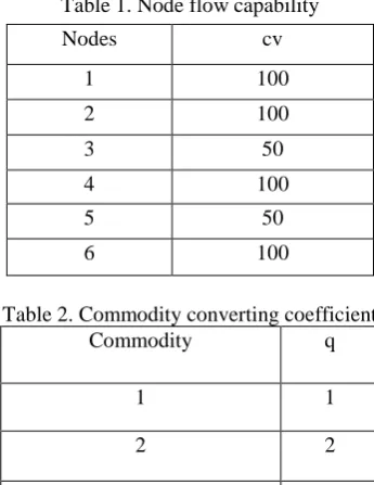
Table 1. Node flow capability
Nodes cv
1 100
2 100
3 50
4 100
5 50
6 100
Table 2. Commodity converting coefficient Commodity q
1 1
2 2
3 3
EAI Endorsed Transactions on
Industrial Networks and Intelligent Systems
5 Table 3: Pairs of source-target nodes
Commodity si,j ti,j
1 1 5
2 2 4
3 3 6
Table 4: Edge capability and cost
Notes: Type 1 is directional, type 0 is undirectional. Edge Type ce be1 be2 be3
(1,2) 1 50 4 5 6
(1,3) 1 50 4 5 6
(2,3) 0 70 4 5 6
(3,2) 0 70 3 4 5
(2,5) 1 50 5 6
(3,4) 1 50 4 5 6
(3,5) 0 70 4 5
(5,3) 0 70 3 5
(4,6) 1 50 4 5 6
(4,5) 0 70 4 6
(5,4) 0 70 3 5
(5,6) 1 50 4 5 6
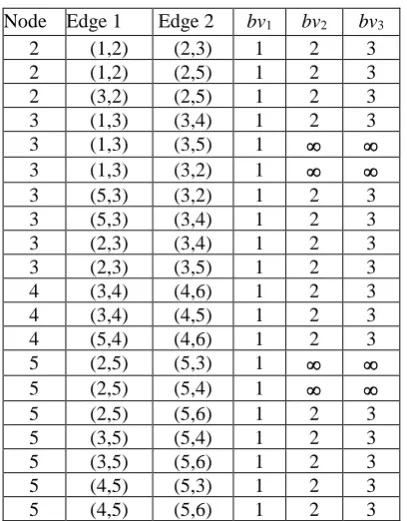
Table 5. Switch cost
Node Edge 1 Edge 2 bv1 bv2 bv3
2 (1,2) (2,3) 1 2 3 2 (1,2) (2,5) 1 2 3 2 (3,2) (2,5) 1 2 3 3 (1,3) (3,4) 1 2 3 3 (1,3) (3,5) 1 3 (1,3) (3,2) 1 3 (5,3) (3,2) 1 2 3 3 (5,3) (3,4) 1 2 3 3 (2,3) (3,4) 1 2 3 3 (2,3) (3,5) 1 2 3 4 (3,4) (4,6) 1 2 3 4 (3,4) (4,5) 1 2 3 4 (5,4) (4,6) 1 2 3 5 (2,5) (5,3) 1 5 (2,5) (5,4) 1 5 (2,5) (5,6) 1 2 3 5 (3,5) (5,4) 1 2 3 5 (3,5) (5,6) 1 2 3 5 (4,5) (5,3) 1 2 3 5 (4,5) (5,6) 1 2 3
The algorithm is coded in C++ and gives correct results. Below is the result of the above example.
Coeficient of approximation:0.070000 Total output: 148.908624
Total cost : 1877.662162
Flow for commodity type 1, which needs to be transferred from source node 1 to destination node 5
1 2 8.396823
1 3 41.500042
2 3 8.396823
3 5 49.896862
Flow for commodity type 2, which needs to be transferred from source node 2 to destination node 4
2 3 0.093091
3 4 0.093091
Flow for commodity type 3, which needs to be transferred from source node 3 to destination node 6
3 2 49.375553
2 5 49.375553
3 4 49.543118
4 6 49.543118
5 6 49.375553
6. Conclusion
The article develops the algorithm finding the shortest path in extended graphs (Section 2), the algorithm finding the shortest path on the multiple-weighted extended graph (Section 3). Based on the duality theory of linear programming, an approximation algorithm with polynomial complexity is developed on the base of the algorithm finding shortest paths in section 2 and 3. This is also the main result of the article. Correctness and algorithm complexity are justified and the algorithm is stored in C++ and given an exact result. The results of this article are the basis for studying the applications of multicomodity multicost flow optimization .
7. References
[1] Naveen Garg, Jochen Könemann: Faster and Simpler Algorithms for Multicommodity Flow and Other Fractional Packing Problems, SIAM J. Comput, Canada, 37 (2), 2007, pp. 630-652.
[2] Xiaolong Ma, Jie Zhou: An Extended Shortest Path Problem with Switch Between Arcs, Proceedings of the International Conference on Engineers and Computer Scientists 2008 Vol IIMECS 2008, 19-21 March, 2008, Hong Kong.
EAI Endorsed Transactions on
Industrial Networks and Intelligent Systems
6 [3] Tran Quoc Chien: Linear multitransport network
calculation, ministerial scientific research, code B2010DN-03-52.
[4] Tran Quoc Chien, Tran Thi My Dung: Applying of algorithm finding the shortest path for maximum multicommodity flow. Journal of Science & Technology, University of Danang, 3 (44) 2011.
[5] Tran Quoc Chien: Applying of algorithm finding the shortest path for maximum simultaneous multicommodity flow. Journal of Science & Technology, University of Danang, 4 (53) 2012. [6] Tran Quoc Chien: Applying of algorithm finding the
shortest path for minimum cost maximum simultaneous multicommodity flow. Journal of Science & Technology, University of Danang, 5 (54) 2012.
[7] Tran Quoc Chien: The algorithm findsing the shortest path in the general graph, Journal of Science & Technology, University of Da Nang, 12 (61) / 2012, 16-21.
[8] Tran Quoc Chien, Nguyen Mau Tue, Tran Ngoc Viet: The algorithm finding the shortest path on the extension graph. Proceeding of the 6th National Conference on Fundamental and Applied Information Technology (FAIR), Proceedings of the Sixth National Conference on Scientific Research and Applying, Hue, 20-21 June 2013. Natural Science and Technology Publishing House. Hanoi 2013. p.522-527.
[9] Tran Quoc Chien: Applying of algorithm finding the fastest path for maximum multi-transport linearity of minimum cost on extension transportation networks, Journal of Science & Technology, University of Da Nang . 10 (71) 2013, 85-91.
[10] Tran Ngoc Viet, Tran Quoc Chien, Nguyen Mau Tue: Optimized Linear Multiplexing Algorithm on Extension Transportation Networks, Journal of Science & Technology, University of Da Nang. 3 (76) 2014, 121-124.
[11] Tran Ngoc Viet, Tran Quoc Chien, Nguyen Mau Tue: The calculation of linear multitransport on transportation network. Proceedings of the 7th National Conference on Fundamental and Applied Information Technology Research (FAIR'7), ISBN: 978-604-913-300-8, Proceedings of the 7th National Scientific Conference on "Fundamental and Applied Research IT ", Thai Nguyen, 19-20 / 6/2014. NXB Natural Science and Technology. Hanoi 2014. p.31-39.
[12] Tran Quoc Chien, Ho Van Hung: The multicommodity multi flow expansion network and the algorithm used to find the maximum flow FAIR-2017, August, 2017.
EAI Endorsed Transactions on
Industrial Networks and Intelligent Systems