HIERARCHICAL CLUSTERING BASED MULTI-DIMENSIONAL POLYGON REDUCTION ALGORITHM FOR LARGE SPATIAL DATA

976 |

P a g e

HIERARCHICAL CLUSTERING BASED

MULTI-DIMENSIONAL POLYGON REDUCTION

ALGORITHM FOR LARGE SPATIAL DATA

Dr. Mamta Dahiya

Department of Computer Science & Engineering, Apeejay Stya University, Gurgaon (India)

ABSTRACT

In this paper, a Hierarchical Clustering based multi dimensional polygon reduction algorithm for large spatial

data sets is proposed. The concept of hierarchical clustering to produce a hierarchy of clusters by considering

density and distance as a core parameters are used. It applies agglomerative approach of hierarchical

clustering to a set of clusters produced until a termination condition is satisfied. The advantage of this

algorithm is to reduce polygon edges with polygon reduction method that helps to save memory as there is

exponential growth of data in spatial datasets. In this approach memory would be very less than the matrix

approach contains reduction line as explained in our earlier algorithm pronounced as 3DCCOM. This

algorithm takes into account the problem of clustering in the presence of physical obstacles while modeling the

obstacles by Reentrant Polygon Reduction Algorithm for better performance.

Keywords: Polygon Reduction, Reentrant Polygon, Hierarchical Clustering, Spatial Data

I. INTRODUCTION

Extraction of meaningful information out of spatial data sets assumes importance especially when these voluminous data sets are growing at an exponential rate. Therefore, spatial data mining has become a potential area for researchers in the last one and half decade. Data mining uses clustering for discovering unknown patterns occurring in the data. Clustering is widely used for pattern recognition [1, 2, 3], data analysis [4], image processing [5, 6] and machine learning [7] etc. It is a core activity associated with spatial data mining carried out with a view to segregate data objects into smaller groups based on some proximity measure. That is, clustering is a process in which similar data objects fall under one group (cluster) such that similarity between the data points in one group (cluster) is very high and similarity between two data points of two different groups (clusters) is negligible. This clearly indicates that for quality clusters the similarity measure must be robust. Estimating similarity between two data points depends entirely on the choice of distance metric.

977 |

P a g e

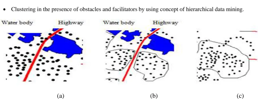
business, astronomical sciences etc. has generated the requirement of tools that can be employed for churning useful and previously unexplored information and knowledge automatically. Moreover, with the abundance of such datasets it has become practically impossible to make them free of noise or outliers. The existing algorithms for clustering expect parameter tuning and provide clusters of arbitrary shapes. These algorithms provide expected results in case of two-dimensional and three-dimensional data sets. Many clustering approaches ignore handling obstacles and facilitators present in spatial datasets, especially GIS that results in inefficient and irrelevant clusters. There are some approaches of spatial data include 3DCCOM [11], COD-CLARANS [13], AUTOCLUST+[10], DBCLUC [15] and DBRS+[16] that can handle obstacles and facilitators together but not their possible combination. Also, the outliers (noise element) in the dataset are determined only as residues (by-products) of the clustering processes. Polygon Reduction clustering algorithm in presence of obstacles, facilitator and constrains which is abbreviated as PRC further extended as a 3DCCOM (Three Dimensional Clustering with Constraints and Obstacle Modelling). 3DCCOM [11] takes into account the problem of clustering in the presence of physical obstacles while modelling the obstacles by Reentrant Polygon Reduction.

As this time, proposed algorithm adopts hierarchical idea to cluster spatial data space in presence of obstacles [12]. It divides the whole data space into multiple regions by keeping two parameters of distance and density parallel without obstacle by raster extension line of obstacle polygon boundary. The presence of obstacles results in the meaningless and impractical spatial cluster result which shows in Fig.1. The problem of spatial clustering in presence of obstacles, facilators and constrains is highly interested recently. Fig.1 (a) shows Original Dataset with obstacles water body and highway etc. (b) formation of cluster with considering obstacles, and (c) showing cluster when ignoring obstacles. In the presented work, the following issues have been significantly addressed:

 Compress/reduce the obstacles i.e. polygons by using set theory.

 Perform clustering without any parameter tuning and human interaction.

 Clustering in the presence of obstacles and facilitators by using concept of hierarchical data mining.

(a)

(b)

(c)

Figure 1 (a)

Original Dataset with obstacles water body and highway etc. (b) Cluster with considering obstacles, (c) cluster when ignoring obstacles

So, a polygon reduction mechanism has been developed to address the challenges stated above.

978 |

P a g e

In literature, various approaches like AutoClust+ [14], COD-CLARANS [13], DBCluC [15], DBRS_O [16] are available that consider the concept of obstacles in the dataset but not many approaches [18] that consider the presence of facilitators also. A facilitator is an object that connects two data objects such as a bridge over a river, a subway under a highway. Conceptually, an obstacle increases the distance between objects while a facilitator decreases the distance. Also, there may be situations in real datasets where two obstacles are intersecting or an obstacle and a facilitator is intersecting or any other possible combination is occurring. The clustering approach must also be able to handle such situation to provide most efficient and relevant clusters.

In COD-CLARANS [13], the authors have represented obstacles through visibility graph and thus computed the obstructed distance between data objects. Also, it detects mostly spherical shaped clusters and depends on user-defined parameters. AutoClust+ [14], which is a graph-based approach, the dataset is modeled through Delaunay structure. DBCluC [15], an extended form of DBSCAN [17], models obstacles using polygons and these polygons are reduced to minimum number of line segments called as obstruction lines that does not compromise with the visibility space. The Fig. 2 shows the obstacle modeling in DBCluc [15]. This approach handles facilitators also, using the concept of entry and exit points.

In [19], a spatial clustering approach in the presence of obstacles based on genetic algorithms and k-medoids has been proposed. Authors have handled obstacles using polygons and visibility graph and thus computed obstructed distance. In [20], a density based clustering with constraints and an obstacle modeling has been proposed. This algorithm uses the concept of polygon reduction but reduction or compressed edges are stored in form of matrix values.

Figure2

. The visibility graph of two data objects a and b having obstacles  and  modeled using polygons.

But in proposed algorithm, compress polygon values are stored using set theory so that use of memory can be more efficient as there is exponential growth in spatial database. We are also using two important parameters: distance and density parallel so that efficient clusters can be formed specifically for demographic data assessment.

2.1

Hierarchical Clustering

979 |

P a g e

2.2

Density Based Clustering

The key idea behind the density based clustering is that for each point of a cluster, the neighborhood of a given radius ( Eps) has to contain at least a minimum number of points (Minpts) i.e. the density of the neighborhood has to exceed some threshold. Following are some definitions to formalize the notion of cluster and noise in the density based clustering.

Definition 2.1

Eps-neighborhood of a point

The Eps-neighborhood of a point p denoted by NEps(p), is defined as: NEps(p)={q ∈D | dist(p,q) ≤ Eps}

Where D is a database of points or objects. Density based clustering require that for each point of a cluster, there should be at least a minimum number of points Minpts in the Eps-neighborhood of that point.

Definition 2.2

Directly-density-reachable

A point q is directly-density-reachable from a point p wrt Eps and Minpts if 1. q ∈ NEps(p) and

2. | NEps(p)| ≥ Minpts

The data points can be divided core points and border points, where core points satisfy density criterion and exist in the core of the dataset, while border points don‟t satisfy density criterion and exist on the borders of the dataset. Eps-neighborhood of a border point contains significantly less number of points than that of a core point. Density based algorithm general idea is to continue growing the given cluster as long as the density in the neighborhood exceeds some threshold i.e. for each data point in the cluster; the neighborhood of a given radius has to contain at least a minimum number of points

Definition 2.3

Density-reachable

A point p is density-reachable from a point q wrt Eps and Minpts if there exists a chain of points p1, p2…pnand p1=q, pn=p, such that pi+1is directly-density-reachable from pi.

Definition 2.4

Cluster

Let D be a database of points. A cluster C wrt Eps and Minpts is a non-empty subset of D satisfying the following conditions:

1. Maximality: ∀p,q∈D, if p∈C and q is density-reachable from p wrt Eps and Minpts, then q∈C.

2. Connectivity: ∀p,q∈C, p and q are density-connected to each other wrt Eps and Minpts.

Definition 2.5

Noise

Let C1, C2…Ckbe the clusters created from the database D wrt Eps and Minpts, then noise is the set of points in the database not belonging to any cluster i.e.

980 |

P a g e

2.3

Dbscan Algorithm

The algorithm DBSCAN (Density Based Spatial Clustering of Applications with Noise) is designed to discover the clusters and the noise in a spatial database in the absence of obstacles according to definitions given above. Ideally, we would have to know the appropriate parameters Eps and MinPts of each cluster and at least one point from the respective cluster. To find a cluster start with an arbitrary point p and retrieve all points density reachable from p wrt Eps and Minpts. If p is a core point, this procedure yields a cluster wrt Eps and MinPts (Lemma 2).

If p is a border point, no points are density-reachable from p and DBSCAN visits the next point of the database. Since we use global values for Eps and MinPts, DBSCAN may merge two clusters according to definition 2.4 into one cluster, if two clusters of different density are “close” to each other. Let the distance between two sets

of pointsS1 and S2 be defined as dist (S1, S2) = min {dist(p,q) | p S1, q S2}. Then, two sets of points having at least the density of the thinnest cluster will be separated from each other only if the distance between the two sets is larger than Eps.

Consequently, a recursive call of DBSCAN may be necessary for the detected clusters with a higher value for MinPts. This is, however, no disadvantage because the recursive application of DBSCAN yields an elegant and very efficient basic algorithm. The most important function used by DBSCAN is ExpandCluster for large dataset. Region queries can be supported efficiently by spatial access methods such as R*-trees or SR trees which are assumed to be available in a SDBS for efficient processing.

2.4

Obstacle Modeling

Almost all physical obstacles like rivers, hills, and highways etc. can be modelled using simple polygons. All the polygons can be divided into two types: simple polygons and crossing polygons. A simple polygon is the polygon in which every edge in the polygon is not intersected with any other edge in the polygon and a crossing polygon is the polygon in which at least one edge is intersected with any other edge in the polygon. Simple polygons can be further divided into two types: convex and concave as shown in figure 3(a) (b). A polygon is a convex polygon if all vertices of the polygon make the same directional turn whether clockwise or anticlockwise. Suppose a polygon P does not follow the claim. It then is obvious that P is not a convex. All other polygons, which don‟t satisfy this condition, are said to be concave. In order to test a turning direction for

3 consecutive vertices, the sign of the triangle area of 3 points is examined via a determinant. As a result, the sign of the determinant evaluates the turning direction either a clockwise or a counter clockwise.

(a) Convex polygon (b) Concave/ Reentrant polygon

All interior

angles are less than 180o

At least one interior angle is

981 |

P a g e

Figure 3(a)

in convex polygon all interior angles are less than 180 degree; (b) in concave polygon at least one

interior angle is greater than 180 degree.

Note that we assume that all points in a polygon are enumerated in an order either clockwise or a counter clockwise. Hence, we can easily identify a type of a polygon as well as a type of each vertex from the polygon in a linear time O (n), where n is the number of points in a polygon.

III. REETRANT POLYGON REDUCTION ALGORITHM

In any clustering algorithms, when obstacles are considered, the visibility of data objects with each other is checked via the line segments or edges of the obstacle. The number of line segments to check is the number of edges of the polygons, which is large in number for a large data space. The number of lines to check can be reduced to actual one by our proposed polygon-edge reduction algorithm but memory would be much less then the matrix approach contains reduction lines. We are here to going to use set of reduction lines. Let us call the

reduced number of lines as reduction lines. The algorithm assumes the following definition of a polygon

.

Definition 3.1:

Polygon

A simple polygon is denoted by an undirected graph P (V, E) where V is a set of k vertices: V = {v1, v2…, vk}

and E is a set of k edges: E = {e1, e2…ek} where ei is a line segment joining vi and vi+1, 1ik. i+1=1 if i+1>k.

First all the convex vertices of the polygon are extracted because only convex vertices are considered to find the visibility between two data objects. Assume that a polygon P (V, E) of n convex vertices is stored in the form of

adjacency matrix A of order n×n where A [I,J]=1 if edge (I,J) exists between vertices I and J i.e.(I,J)  E.

A [I, J] =0 if (I, J) not  E.

The algorithm returns the output ordered set O.

O = {(I, J): I, J ɛV, pair (I, J) is a reduction line}

It first identifies the convex vertices in the polygon by turning direction approach and by checking the triangle area of three consecutive points via its determinant. After finding all the n convex vertices, a matrix A of order n×n stores the link information about polygon. The entries in the upper half of matrix „A‟ are checked so as to avoid the repetition because the polygon is undirected graph.

Algorithm: Reentrant_poly_red (P)

//P is given polygon with V vertices and E edges

//Output: A set of obstruction lines (I, J) in ordered set O. Identify the convex and concave vertices. Let convex vertices be n; Store the link information of convex vertices in A taking them in order;

Flag=0; k=0;

FOR (I=1; I<=n; I++) {

982 |

P a g e

{ // B is matrix for storing row numbers

Flag: =1; }

FOR (J=I; J<=n; J++) {

IF( ( A[I,J]= =1) OR ( (A[I,J]= =0) AND ( (I,J) is interior to P) )) {

Push (O, I, J); // Insert (I, J) into ordered set O B[k]:=J; k++;

}

IF (Flag = = 1) {

A [I, J]:=0; } }

Flag: =0; } }

Return O i.e. Reduction Lines L; // END

All reduction lines should be interior to polygon P and each convex vertex should‟ve at least one reduction line

from it. The number of reduction lines must be at least equal to the number of convex vertices to allow the correct visibility between the data points. Take the example convex polygon shown in figure 4(a) that has six convex vertices and six edges. Corresponding to these six convex vertices, the input matrix A becomes as shown in figure 4(b). As a result of the application of the polygon reduction algorithm, the output ordered set O is shown in figure 4(d). The output-reduced polygon is constructed according to output ordered set O and is shown in figure 4(c), which contains five instead of six reduced lines.

1 2

6 3

5

4

(a) Input Polygon

(b) Input matrix A(with replicated values)

1 2 3 4 5 6

1

0

1 0 0 0 1

983 |

P a g e

1

2

6 3

Set(O)={ (1,2) (1,3) (1,4) (1,5) (1,6) }

5 4

(c) Output Matrix

(d) Output ordered set O

Figure 4 (

a) Input Polygon, (b) Input Matrix A having replicated data, (c) Output Matrix, (d) Output ordered set O with no replicated data

This is the case where significant improvement is not achieved but in the case of concave polygons, a remarkable improvement can be obtained. So, in a large dataset, where the number of obstacles can be large in number and hence the number of edges to test is also large in number, the polygon reduction algorithm can be applied to reduce the number of lines to test during the clustering procedure.

IV. PROPOSED ALGORITHM

PROPOSED HIERARCHICAL CLUSTERING BASED MULTI DIMENSIONAL POLYGON REDUCTION ALGORITHM FOR

LARGE SPATIAL DATA SETS IS BASED ON 3DCCOM (3 DIMENSIONAL CLUSTERING WITH CONSTRAINTS AND

OBSTACLE MODELLING)[11] PRONOUNCED AS 3DCCOM TAKES INTO ACCOUNT THE PROBLEM OF CLUSTERING IN

THE PRESENCE OF PHYSICAL OBSTACLES WHILE MODELLING THE OBSTACLES BY POLYGON REDUCTION. THE

ALGORITHM ALSO USING CONCEPT OF DENSITY BASED CLUSTERING. IT APPLIES AGGLOMERATIVE APPROACH OF

HIERARCHICAL CLUSTERING TO A SET OF CLUSTERS PRODUCED UNTIL A TERMINATION CONDITION IS SATISFIED.

DISTANCE AND DENSITY ARE TWO KEY PARAMETER FOR PROPOSED ALGORITHM. TO BETTER HAVE AN UNDERSTANDING OF THIS, WE HAVE ANOTHER DEFINITION TO FIND THE DISTANCE BETWEEN THE TWO CLUSTERS.

Definition 4.1

Distance between two clusters

Let C = {c1, c2…ck} be the set of clusters produced by any clustering algorithm. The distance between two clusters ci and cj is defined as: dist (ci, cj) = Min {dist (p, q) | p Є ci and q Є cj}.

The distance function takes all the points from two clusters and finds the distance, which is the distance between two nearest neighbors respectively from two clusters as Fig. 5 below shows.

984 |

P a g e

The threshold distance Dmin is taken to have an upper bound on the acceptable distance between two clusters. Two clusters can be merged at a subsequent step if the distance between the two clusters is no more than Dmin but we also keep density of cluster as an important parameter. The clusters at subsequent steps are merged together until the current clustering at a stage becomes similar to the clustering at the previous stage i.e. the

number of clusters is same at two stages; this forms the termination condition for the proposed algorithm

.

Proposed_

algorithm (Database D, obstacles O, Dmin)

// Dmin is the minimum threshold distance between two clusters c1 and c2; Dmin>Eps //Output: A hierarchy of Clusters with distance and density parameter

C: = 3DCCOM (D, O); //Start clustering as in 3DCCOM DO

FOR (D=DT; D<= Dmax; D=D+DT)

FOR (random ci and cj set of clusters C) do

IF (DciD) AND (DcjD) AND (dist (ci,cj)Dmin ) // D is aligned threshold density Pts: =merge (ci,cj);

ClusterId:= assign_next_Id(pts,ClusterId); Density of ClusterId=Dci+Dcj

Add ClusterId to C‟;

Remove ci,cj from set of clusters C; END IF;

ELSE

Remove ci,cj from set of clusters C; Add ci, cj to C‟;

END ELSE; END FOR; END FOR;

Write ClusterIds of clusters in C‟ to C;

WHILE //(no more change from previous clustering); RETURN// hierarchy of clusters;

One example illustrating this idea, in this figure 5= {p1, p2… p10} is the original clustering produced by the clustering algorithm wrt Eps and Minpts and is at level 1. Further merging of clusters result at level 2. In this way process goes up to level 8, which may be similar to level 9, where process of hierarchical clustering stops.

V.

EXPERIMENTAL RESULTS AND ANALYSIS OF PROPOSED ALGORITHM

985 |

P a g e

between algorithms, the real data set is used and compares it with new dataset. For simplicity, the synthetic spatial data set is 3-dimesional spatial data. The data set and obstacles are showed as Fig.6 (a). The best results of algorithms with a broad range of parameter settings are selected. Clustering result of this spatial data space is showed by Fig.6 (b), (c), and (d) when the obstacles, facilitator, outliers are present or ignored. The simulated results are shown with help of ArcGIS tool. The different cluster of data space is described by different color as following.

`(a)

(b)

(c)

(d)

Figure 6 (a)

Population distribution considering obstacles and facilitators of Rohat Village, Sonepat, India, (b) Population Clusters with a fixed densities, (c) Population clusters with proposed Algorithm at

level 3 and (d) clusters at level 4

986 |

P a g e

of facilitator and obstacles than DBCLUC. DBCLUC can cluster spatial data space with obstacles, but the process of obstacles in arbitrary shape is ideal insufficiently.

We can find out heterogeneous or homogeneous population distribution per capita by ignoring or considering different obstacles and facilitators. Here with proposed algorithm Cluster results in presence of obstacles and constrains are showed by Fig 6 (b) Population Clusters with a fixed densities, fig 6(c) Population clusters at level 3, and fig 6 (d) Population clusters with proposed algorithm at level 6 in the Presence of obstacles and facilitators. Through comparison and analysis of cluster results of two algorithms, the conclusion is that proposed algorithm can get better cluster result in presence of facilitator and obstacles than DBCLUC. DBCLUC can cluster spatial data space with obstacles, but the process of obstacles in arbitrary shape is ideal insufficiently. There are many scattered meaningless cluster in the final cluster result of DBCLUC.

Algorithm proposed in this paper inherits advantage of polygon reduction and density cluster algorithm and it can operate obstacle polygons and find clusters in arbitrary shape to avoid scattered meaningless cluster in final result. So the cluster result of proposed algorithm is more accurate and more practical. At the same time, the execution space-time cost of this algorithm is very less than DBCLUC because of the adoption of reentrant polygon reduction strategy using set theory.

There are a number of areas into which the proposed work can be extended or improved. The work shows how to consider obstacles in the clustering process and how to model the physical obstacles using the reduction algorithm, but no indexing scheme is used for obstacles. In the absence of any indexing scheme, all produced reduction lines are checked for visibility of a data point. By using an indexing scheme, only lines in the neighborhood of a particular data point can be checked instead of all the lines. With such a scheme, the complexity can be reduced to O (N log N) which would be a significant improvement over the proposed algorithm.

VI. ACKNOWLEDGMEN

T

The authors would like to thank the Apeejay Stya University to support me in research and allow me to use laboratory for various software.

REFERENCES

[1] Yeung K. Y., Fraley C., Murua A., Raftery A. E., and Ruzzo W. L.(2001): Model-based clustering and data transformations for gene expression data. Bioinformatics, 17(10):pp.977–987.

[2] Law M. H. C., Topchy A. P., and Jain A. K.(2004): Model-based clustering with soft and probabilistic constraints. Technical report, Michigan State University.

[3] Zhong S. and Ghosh J.(2003), A Unified Framework for Model-based Clustering Data Analysis. In Journal of Machine Learning Research, pp. 1001-1037 .

987 |

P a g e

[5] Yixin C., James Z., Wang and Robert K.(2005): CLUE: Cluster-based Retrieval of Images by Unsupervised

Learning. IEEE Transactions on Image Processing, vol. 14, no. 8, pp. 1187-1201.

[6] Schmid P.(2001): Image segmentation by color clustering, http://www.schmid-saugeon.ch/publications.html.

[7] Zhang Y.F., Mao J.L., Xiong Z.Y.(2003), An efficient clustering algorithm. In Proc. of Intl. Conf. On Machine learning and Cybernetics, pp. 261-265, Vol. 1.

[8] www-users.cs.umn.edu/~kumar/papers/high_dim_clustering_19.pdf

[9] www.ucl.ac.be/mlg/index.php?page=PartTop&WhichTop=5

[10] V. Estivill Castro, I. J. Lee, 2000 “AutoClust+: Automatic Clustering of Point-Data Sets in the Presence of Obstacles,” Int. Workshop on Temporal, Spatial and Spatio-Temporal Data Mining, pp. 133-146.

[11] Mamta Malik, Dr. Parvinder Singh, and Dr.A.K.Sharma, “3DCCOM Polygon Reduction Algorithm in Presence of Obstacles, Facilators and Constraints” in International Journal of Computer Applications

29(7):6-12, September 2011. Published by Foundation of Computer Science, New York, USA.

[12] Yue Yang, Jian-pei Zhang, Jing Yang, 2008, Grid-based Hierarchical Spatial Clustering Algorithm in Presence of Obstacle and Constraints” at International Conference on Internet Computing in Science and

Engineering.

[13] Tung A.K.H., Hou J., and Han J.(2001): Spatial Clustering in the Presence of Obstacles. In Proc. of Intl. Conf. on Data Engineering (ICDE'01), Heidelberg,Germany, pp. 359-367.

[14] Estivill-Castro V. and. Lee I.J.( 2000): AUTOCLUST+: Automatic Clustering of Point-Data Sets in the Presence of Obstacles. In Proc. of the Intl. Workshop on Temporal, Spatial and Spatial-Temporal Data Mining, Lyon, France,. pp. 133-146.

[15] Zaïane O. R., and Lee C. H. (2002): Clustering Spatial Data When Facing Physical Constraints. In Proc. of the IEEE International Conf. on Data Mining, Maebashi City, Japan, pp.737-740.

[16] Wang X. and Hamilton H.J.(2004): Density-based spatial clustering in the presence of obstacles. In Proc. of 17th Intl. Florida Artificila Intelligence Research Society Conference (FLAIRS 2004), 312-317, Miami.

[17] Wang W.,Yang J., Muntz R.R.(1997): STING: A statistical information grid approach to spatial data mining. In Proc. of 23rd Conference on VLDB, 186-195, Athens, Greece.

[18] Wang X., Rostoker C., .Hamilton H.J.(2004): Density-Based Spatial Clustering in the Presence of Obstacles and Facilitators. In Proc. of the 8th European Conference on Principles and Practice of Knowledge Discovery in Databases (PKDD 2004), Italy, pp.446-458.

[19] Tung A.K.H., Han J., Lakshmanan L.V.S. and Ng R.T.(2000): Geo-Spatial Clustering with User-specified Constraints. In Proc. of the Intl. Workshop on Multimedia Data Mining(MDM/ KDD‟2000) , Boston, USA.