Numerical Simulation Of A Highly Maneuvering
Target In 2D Using The Bayesian Framework
Radhika MN, S S Parthasarathy, Mahendra Mallick
Abstract: In this paper we describe numerical simulation of a highly maneuvering target in 2D using the Bayesian framework. We consider accelerations of 3g, 4g, and 5g for the highly maneuvering target using the nearly constant turn (NCT) motion in the counter-clockwise and clockwise directions. The target has a sequence of nearly constant velocity (NCV) and NCT motions. We simulate true trajectories of the target in Monte Carlo runs using the prior distribution and the NCV and NCT dynamic models. A fixed moving target indicator (MTI) radar is used to generate range, azimuth, and radial velocity measurements.
Keywords: Bayesian framework, Highly maneuvering target, Monte Carlo simulation, Nearly constant turn (NCT), MTI radar measurement model —————————— ◆ ——————————
1.
INTRODUCTION
Two commonly used frameworks in filtering are the Bayesian and Fisher frameworks [1], [6], [12], [28], [29], [31], [32]. The state of the target in the Bayesian framework is a random variable, whereas the state of the target in the Fisher framework is non-random. At present the Bayesian framework is regarded as the preferred model for filtering [1], [6], [28], [31], [32].
A filtering algorithm has a dynamic model and a measurement model. The dynamic model describes the motion of the target and the measurement model describes the relationship of the measurement on the target state and measurement noise. The famous Kalman filter (KF) algorithm [14] is based on the Bayesian framework. In the KF, the dynamic and measurement models are linear with additive zero-mean white Gaussian process and measurement noises [1], [6]-[8], [14], [28]. In addition, the initial state has a prior Gaussian distribution with known mean and covariance [1], [28], [31]. The initial state, the process noise, and measurement noise are assumed as independent [1], [6-7], [28], [31]. The KF is an optimal estimator in the minimum mean square error (MMSE) sense [1], [6-7], [28] under standard KF assumptions. However, many real-world problems are nonlinear in nature. The KF is not applicable to problems when the dynamic or/and measurement models are nonlinear [1], [6-8], [28]. An optimal filtering algorithm in the MMSE sense does not exist for a nonlinear filtering problem [1], [6-7], [28]. A number of approximate nonlinear filters have been proposed for nonlinear filtering problems. Commonly used nonlinear filtering algorithms are the extended Kalman filter (EKF) [1], [6-8], [20], [21], [28], [30], unscented KF (UKF) [13], [21], [28], cubature KF (CKF) [2], and particle filter (PF) [3-4], [28]. A maneuvering target is an accelerating target [19]. A non-maneuvering target moves with constant velocity (CV) or nearly CV (NCV) [6-7], [19]. For an accelerating target, the speed, direction of velocity, or both can change. Examples of a maneuvering target motion with one type of dynamic model are motions with nearly constant acceleration (NCA) and nearly constant turn (NCT) [4], [6-7], [19], [28]. In real-world scenarios, a target can move with multiple motions, such as a sequence of NCV, NCA, NCT, NCV, etc. [15], [21]. In such cases, a filtering algorithm using a single dynamic model is not applicable. A famous algorithm for a maneuvering target with multiple motion models is the interacting multiple model (IMM) estimator [6-8], [10-11], [21], [25], [28], which uses a fixed
number of dynamic models for the full observation period.
When the number of dynamic models is high, improved filtering accuracy can be achieved by adaptively selecting a subset of the dynamic models as is done in the variable-structure IMM (VS-IMM) filter [17-19]. Typically, a highly maneuvering target can have an acceleration of greater than 2g [5], [9], [16], [27], where g is the acceleration due to gravity with a nominal value of The acceleration of a target can be expressed in terms of the g-factor. Since the acceleration will depend on the type of target, it is important to consider the type of target while simulating trajectories of a target. Highly maneuvering targets can be ballistic missiles, cruise missiles, interceptors, or fighter aircraft. The speeds of a cruise missile and ballistic missile are around 1500 m/s and 5000 m/s, respectively. Bahari et al. [5] considered a target moving with constant acceleration, and the maximum acceleration had a value of about 3.2 g. In [9] Blackman et al. considered a highly maneuvering aircraft with a maximum acceleration of 3g moving with the NCT motion. Kumar et al. [16] studied interception of highly maneuvering targets using seeker-less interceptors. Accelerations of the interceptors in their study were 2g and 4g. Meng et al. [27] analyzed a low altitude (30 km) target moving in Earth’s atmosphere under the influence of Earth’s spherical gravitational field and atmospheric drag. The numerical value of the acceleration of the target is not available in this paper. Yang and Ji [33] studied a highly maneuvering aircraft with the NCA motion which had a maximum acceleration of about 3.7 g. In this paper we consider a fighter aircraft whose speed is around 370 m/s and which can have accelerations of 3g, 4g, or 5g. For simplicity we have assumed that the target moves in 2D (plane) and consider a fixed MTI radar [20-22] in the XY-plane. In realistic scenarios, the target and radar can move in 3D in different planes as considered in [24]. In many published papers and books, the measurement function for azimuth is not correctly stated, and the domain of the azimuth measurement function is used as the real line Stated correctly, the domain and range of the azimuth measurement function are and respectively. Our previous work in [23] has clearly explained this issue.
The main objectives of this paper are:
• Clearly describe simulation of true trajectories in Monte Carlo runs using the Bayesian framework.
3263 • Simulate true trajectories for a highly maneuvering target
using accelerations of 3g, 4g, and 5g.
• Explain variations of range, azimuth, and radial velocity with time as the target moves with NCV and NCT motions. • Specifically, explain variation of azimuth in the interval
We use “:=” to define a quantity. An italic letter denotes a scalar quantity and a boldface lower or upper case Roman letter denotes a vector or a matrix. The transpose of a vector or matrix A is denoted as “ ”The organization of the paper is as follows. Sections 2 and 3 present the dynamic and measurement models. For circular motion in 2D, we present relationships among speed, angular velocity, and centripetal acceleration in Section 4. Section 5 presents numerical simulations and results, and section 6 summarizes our contributions in the paper and discusses future work.
2.
DYNAMIC MODELS
In this paper we consider the motion of a target in 2D. This section discusses in detail the discrete-time dynamical models used to represent different target motions for a highly maneuvering target. These motions are the NCV and NCT motions in clockwise and anti-clockwise directions. There are two types of discrete-time dynamic/kinematic models, discretized continuous-time model and direct discrete-time model [6]. We follow the discretized continuous-time model, since this naturally follows from Newton’s second law. The position and velocity components of the target state are denoted by and , respectively. The state vector of the target at time for both the NCV and NCT model is defined by [4], [28]
(1)
We refer to the NCV, NCT in the anti-clockwise direction, and NCT in the clockwise direction as models 1, 2, and 3, respectively. The model index is used as a superscript in the state transition matrix, process noise, and process noise covariance matrix. 2.1.Nearly Constant Velocity Model The dynamic model for the NCV motion is described by [1], [6-7], [20] (1) (1) 1 1 1 k k k k
x
=
F
−x
−+
− (2)where is the state transition matrix is the integrated process noise (we shall use “process noise” for simplicity) in the time interval [6], [20]. We assume that the process noise is zero-mean, white, Gaussian with covariance The state transition matrix and process noise are described by [6], [20] (1)
1
1
0
0
0
1
0
0
0
1
0
0
0
0
1
kT
T
F
−=
(3)(4)
(5)
(6)
where is the Kronecker delta, is the power spectral density (PSD) of the X or Y components of the continuous-time acceleration process noise [6], [20]. 2.2.Nearly Constant Turn Model The dynamic models for the NCT motions are described by [4], [6], [28] (7)
where the state transition matrices are given by (8)
(9)
where is typical maneuver acceleration and are 1 and -1 corresponding to counter-clockwise and clockwise NCT motions, respectively. The process noise covariance matrices are (10) where and are the PSD of the process noise for models 2 and 3, respectively [4], [6], [28]. We use
3.
MEASUREMENT MODEL
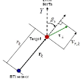
A moving target indicator (MTI) radar measures the range, bearing (or azimuth), and radial velocity of the target [20-22], [24]. We assume that the radar is at a fixed position Let and denote the position and velocity of the target at time (11)(12)
The range vector at time is given by (13)
where represents the norm of the range vector. The unit vector along the radar line-of-sight (LOS) or the range vector is defined by
(15)
The radial velocity of the target is defined as the projection of the target velocity along the RLOS as shown in Fig. 1 and is given by [20-22], [24] (16)
Let be the angle between the velocity of the target and the RLOS at time (see Fig. 1). Then the radial velocity at time an also be written as , (17)
where is the speed of the target at time Fig. 1 defines the true range, azimuth, and radial velocity of the target at time Figure 1. Definition of true range, azimuth, and radial velocity. From Fig. 1 and (17), we find that when the target velocity is along or opposite to the RLOS, the radial velocity has the maximum and minimum values of and respectively. The radial velocity is zero when the target velocity is perpendicular to the RLOS. Let denote the measurement of the MTI radar at time . The measurement model for the MTI radar is described by [20-22], [24] (18)
where (19)
(20)
(21)
where h is the nonlinear measurement function and is a zero-mean white Gaussian measurement noise with covariance (22)
(23)
(24)
(25)
where are the standard deviations (SDs) of range, azimuth, and radial velocity, measurement errors, respectively. 3.1. Remark on Azimuth Measurement Function We note that in (21), and lie in Therefore, the domain and range of the azimuth measurement function are and respectively, as explained in [23]. For the azimuth measurement function, many published papers and books use (26)
In (26), the domain and the range of the azimuth measurement function are and respectively, and hence do not represent correct results. In sub-section 5.5.2, we clearly describe the variation of the azimuth measurement function for the 4g acceleration scenario in the range .
4.
RELATIONS AMONG SPEED, ANGULAR
VELOCITY, AND ACCELERATION
Consider a target moving in a plane in a circular arc of radius with constant speed and constant angular velocity Let be the centripetal acceleration of the target. Then we havev
=
R
(27)(28)
Suppose the direction of velocity changes by an amount during time interval Since the angular velocity is constant, (29)
Therefore, from (28) and (29) we get (30)
Suppose in 60 seconds, and Using
(29), the speed is about 374.332 m/s. We have used this value for the constant speed in all three scenarios where the target accelerations are and The values of acceleration, speed, angular velocity, and radius of the arc are shown in Table 1 for these three scenarios.
Table 1. Variation of angular velocity and radius with acceleration.
Acceleration Speed (m/s)
3265
5.
NUMERICAL SIMULATION AND RESULTS
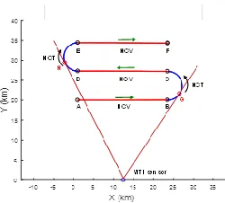
We consider a highly maneuvering target moving in 2D. The target can have an acceleration of 3g, 4g, or 5g during the NCT motion as shown in Figs. 2, 3, or 4, respectively.
5.1. Target Parameters
The prior mean and variance of the target and PSD of the process noise for the NCV and NCT motions are shown in Table 2.
Table 2. Parameters of target. Variable Value Prior mean position (1000, 20000) m Prior mean velocity (374.332,0)m/s Variance of prior position
Variance of prior velocity
NCV: PSD of process noise 0.1 NCT: PSD of process noise 0.01
From Table 1, let and represent angular velocities of 4.5, 6.0, and 7.5 deg/s for the 3g, 4g, or 5g acceleration scenarios, respectively. Motion types in various segments shown in Figs. 2, 3, and 4 are summarized in Table 3.
Table 3. Type of motion in different segments.
Segment
Time Duration
(s)
Type of Motion
AB 60 NCV 0
BC 30 NCT
CD 60 NCV 0
DE 30 NCT or
EF 60 NCV 0
Figure 2. True target trjectory from the first Mont Carlo run with 3g and -3g accelations and MTI sensor position.
Figure 3. True target trjectory from the first Mont Carlo run with 4g and -4g accelations and MTI sensor position. The LOS is tangent to the circular arc at G and H. Thus, the radial
velocity has local maxima at G and H.
Figure 4. True target trjectory from the first Mont Carlo run with 5g and -5g accelations and MTI sensor position.
5.2. Prior Distribution
Figs. 5 and 6 show the initial position and velocity components, respectively, from 500 Monte Carlo runs using the prior distribution.
Figure 5. Initial X and Y coordintaes from 500 Monte Carlo runs using the prior distribution of position.
5.3. MTI Radar Parameters
Table 4 presents MTI sensor position and measurement parameters.
Table 4. MTI radar and measurement parameters. Variable Value MTI radar position (12500, 0) m
Range SD 10 m
Azimuth SD 0.001 rad
Radial velocity SD 1 m/s
Measurement time interval 0.5 s
Number of measurements 481
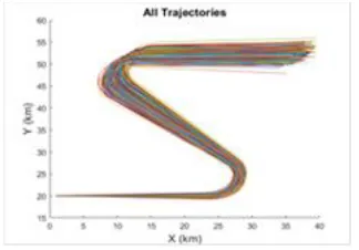
5.4. True Trajectories
Target true trajectories from 500 Monte Carlo runs for 3g, 4g, and 5g accelerations are presented in Figs. 7, 8, and 9, respectively. We observe from Figs. 7-9 that there is a small spread of positions at the
Figure 7. True target trajectories for 3g acceleration from 500 Monte Carlo runs.
initial time due the prior distribution. The spread among the trajectories gradually increases with time due to process noise and nonlinear dynamic models.
Figure 8. True target trajectories for 4g acceleration from 500 Monte Carlo runs.
Figure 9. True target trajectories for 5g acceleration from 500 Monte Carlo runs.
5.5. MTI Sensor Measurements
We have chosen the scenario for the 4g acceleration to present plots for the range, azimuth, and radial velocity measurements.
5.5.1. Range Measurements
Fig. 10 presents range measurements corresponding to 500 Monte Carlo runs in Fig. 3.
Figure 10. Range measurement for 4g acceleration from 500 Monte Carlo runs.
We present Fig. 11 with the beginning and end points of various segments to explain the variation of range with the measurement index in the first Monte Carlo run. As the target moves from A to B in in Fig. 3 with the NCV motion, the range decreases and reaches its minimum when the target is right above the MTI sensor. Then the range gradually increases as the target moves to B and reaches a local maximum at a point before the end point of the arc BC. Next, the range decreases as the target moves towards D and at the midpoint of CD, it has a local minimum. Similar variations in range are explained as the target moves from midpoint of CD to D, then to E, midpoint of EF, and F. Three local minima of range in Fig. 11 correspond to midpoints of segments AB, CD, and EF. Two local maxima of range in Fig. 9 appear before the end points of arcs BC and DE.
3267 5.5.2. Azimuth Measurements
Azimuth measurements for the 4g acceleration scenario from 500 Monte Carlo runs are presented in Fig. 12. To explain the variation of azimuth with the measurement index, we present Fig. 13 with the beginning point of AB, midpoints of AB, BC, CD, DE, and EF, and the end point of EF. When the target is at A, the azimuth has a value of about 330 deg. As the target moves from A towards the midpoint of AB, the azimuth gradually increases to a value close to 360 degrees at just before the midpoint of AB. At just after the midpoint of AB, the azimuth has a value close to zero. As the target moves from the midpoint of AB to the midpoint of the arc BC, the azimuth gradually increases and reaches a local maximum at As the target moves from to the midpoint of CD, the azimuth gradually decreases to zero at a point just before the midpoint of CD. Right after the midpoint of CD at
the azimuth is closer to 360 degrees. As the target moves to the midpoint of the arc DE, it reaches a local minimum. As the target moves from to the midpoint of EF, the azimuth reaches a value close to 360 degrees at a point just before the midpoint of EF. Right after the midpoint of EF at the azimuth is close to zero. After the midpoint of EF, the azimuth gradually increases as the target moves to F.
Figure 12. Azimuth measurements for 4g acceleration from 500 Monte Carlo runs.
Figure 13. True azimuth measurements for 4g acceleration from the first Monte Carlo run.
5.5.3. Radial Velocity Measurements
Fig. 14 presents radial velocity measurements for the 4g acceleration scenario from 500 Monte Carlo runs. For clarity of interpretation, we have presented radial velocity measurements for the 4g acceleration
Figure 14. Radial velocity measurements for 4g acceleration from 500 Monte Carlo runs.
scenario from the first Monte Carlo run in Fig. 15. At point A, the angle between the target velocity and RLOS is greater than 90 degrees. Therefore, the target velocity has a negative component along the RLOS and the radial velocity at A is negative. As the target moves from A to the midpoint of AB, the radial velocity changes from a negative value to about zero. When the target moves from the midpoint of AB towards B, the angle between the target velocity and RLOS decreases and the radial velocity become more positive. From Fig. 3, the RLOS is tangent to the circular arcs BC and DE at G and H, respectively. Therefore, the target velocity and RLOS are parallel at these points. The radial velocity has local maxima at G and H. In Fig. 16, we have plotted the angle between the velocity and RLOS from the first Monte Carlo run. We observe from Fig. 16 that at G, the angle between the velocity and RLOS is nearly zero degrees. As the target moves from G to C the radial velocity decreases. The variation of radial velocity is similarly explained as the target moves from C to D, H, E, and F.
Figure 16. Angle between the velocity and RLOS from the first Monte Carlo run.
6.
CONCLUSIONS
In this paper, we described details of the numerical simulation of a highly maneuvering target in 2D using the Bayesian framework. In our scenarios; the target can have accelerations of 3g, 4g, or 5g. The target has a sequence of nearly constant velocity (NCV) and nearly constant turn (NCT) motions. We used a fixed moving target indicator (MTI) radar to generate range, azimuth, and radial velocity measurements. In our simulation, 500 Monte Carlo runs were used to generate true trajectories and MTI sensor measurements. Our future work will focus on dynamic state estimation of a highly maneuvering target and performance evaluation of filtering algorithms for the problem.
7 REFERENCES
1. B. D. O Anderson and J. B. Moore. Optimal Filtering, Courier Corporation, 2012.
2. Arasaratnam and S. Haykin, “Cubature Kalman filters,” IEEE Transactions on Automatic Control, vol. 54, no. 6, pp. 1254–1269, Jun. 2009.
3. S. Arulampalam, S. Maskell, N. Gordon, and Tim Clapp. "A tutorial on particle filters for online nonlinear/non-Gaussian Bayesian tracking." IEEE Transactions on Signal Processing, vol. 50, no. 2, pp. 174-188, 2002. 4. S. A. Arulampalam, B. Ristic, N. Gordon, and T. Mansell,
"Bearings-only tracking of manoeuvring targets using particle filters," EURASIP Journal on Applied Signal Processing, pp. 2351-2365 2004.
5. M. H. Bahari, N. Pariz, S. M. Davarpanah, and S. Toosizadeh. "An Intelligent Self-Tuning Approach for High Maneuvering Target Tracking." Proc. 2009 Second International Conference on Computer and Electrical Engineering, vol. 2, pp. 249-253, 2009.
6. Y. Bar-Shalom, X. R. Li, and T. Kirubarajan, Estimation with Applications to Tracking and Navigation, New York, NY, USA, Wiley, 2001.
7. Y. Bar-Shalom, P. Willett, and X. Tian, Tracking and Data Fusion: A Handbook of Algorithms, YBS Publishing, 2011. 8. S. Blackman and R. Popoli, Design and Analysis of
Modern Tracking Systems, Artech House, 1999.
9. S. S. Blackman, R. J. Dempster, B. Blyth, and C. Durand, “Integration of Passive Ranging with Multiple Hypothesis Tracking (MHT) for Application with Angle-Only Measurements,” Proc. of SPIE, vol. 7698, pp. 769815-1 – 769815-11, 2010.
10. H. A. P. Blom, “An efficient filter for abruptly changing systems,” Proc. 23rd IEEE Conference on Decision and Control, pp. 656-658, Las Vegas, NV, Dec. 1984.
11. H. A. P. Blom, and Y. Bar-Shalom, “The Interacting Multiple Model algorithm for systems with Markovian switching coefficients,” IEEE Transactions on Automatic Control, vol. 33, no. 8, pp. 780-783, Aug., 1988.
12. G. D'Agostini, Bayesian reasoning in high-energy physics: principles and applications, No. CERN-99-03. Cern, 1999. 13. S. Julier, J. Uhlmann, and H. F. Durrant-Whyte, A new
method for the nonlinear transformation of means and covariances in filters and estimators,” IEEE Transactions on Automatic Control, vol. AC-45, no. 3, pp. 477–482, Mar. 2000.
14. R. E. Kalman, “A New Approach to Linear Filtering and Prediction Problems,” Transaction of the ASME—Journal of Basic Engineering, pp. 35-45, March 1960.
15. T. Kirubarajan, and Y. Bar-Shalom, K. R. Pattipati, and I. Kadar, “Ground Target Tracking with Variable Structure IMM Estimator,” IEEE Transactions on Aerospace and Electronic Systems, vol. 36, no. 1, pp. 26-46, Jan. 2000. 16. G. S. Kumar, D. Ghose, and A. Vengadarajan, “An
integrated estimation/ guidance approach for seeker-less interceptors,” Proc. of the Institution of Mechanical Engineers, Part G: Journal of Aerospace Engineering, vol. 229, no. 5, pp. 891-905, 2015.
17. X. R. Li and Y. Bar-Shalom, “Multiple-Model estimation with variable structure,” IEEE Transactions on Automatic Control, vol. 41, no. 4, pp. 478-493, 1996.
18. X. R. Li, “Engineer’s Guide to Variable-Structure Multiple-Model Estimation for Tracking,” in Multitarget-Multisensor Tracking: Applications and Advances, Volume III, Ed. Y. Bar-Shalom and W. D. Blair, pp. 449-567, Aetech House, 2000.
19. X. R. Li and V. Jilkov, “Survey of maneuvering target tracking," IEEE Trans. Aerospace and Electronic Systems, vol. 39, no. 4, pp. 1333-1364, 2003.
20. M. Mallick and S. Arulampalam, “Comparison of nonlinear filtering algorithms in ground moving target indicator (GMTI) target tracking, Proc. SPIE, vol. 5204, Aug. 2003, pp. 630–647.
21. M. Mallick and B. F. La Scala, “IMM for Multi-sensor Ground Target Tracking with Variable Measurement Sampling Intervals” Proc. 9h International Conference on Information Fusion, Florence, Italy, Jul. 2006.
22. M. Mallick, Y. Bar-Shalom, T. Kirubarajan, and M. Morelande, “An Improved Single-Point Track Initiation Using GMTI Measurements,” IEEE Transactions on Aerospace and Electronics Systems, vol 51, no. 4, pp. 2697-2714, Oct. 2015.
23. M. Mallick, “A Note on Bearing Measurement Model,”
ResearchGate, May 2018, DOI:
10.13140/RG.2.2.13441.35681.
24. M. Mallick, K-C. Chang, S. Arulampalam, and Y. Yan, “Heterogeneous Track-to-Track Fusion in 3D Using IRST Sensor and Air MTI Radar,” IEEE Transactions on Aerospace and Electronics Systems, Feb. 2019, DOI 10.1109/TAES.2019.2898302.
25. E. Mazor, A. Averbuch, Y. Bar-Shalom, and J. Dayan, " Interacting Multiple Model Methods in Target Tracking:A Survey," IEEE Transactions on Aerospace and Electronic Systems, vol. 34, no. 1, pp: 103-123, Jan. 1998.
26. L. A. McGee and S. F. Schmidt, "Discovery of the Kalman filter as a practical tool for aerospace and industry," 1985. 27. Q. Meng, B. Hou, D. Li, Z. He, and J. Wang,
"Performance Analysis and Comparison for High Maneuver Target Track Based on Different Jerk Models," Journal of Control Science and Engineering, 2018.
28. B. Ristic, S. Arulampalam, and N. Gordon, Beyond the Kalman Filter, Artech House, 2004.
29. C. Robert, The Bayesian Choice: From Decision-Theoretic Foundations to Computational Implementation, Springer Science & Business Media, 2007.
3269 Guidance, Control, and Dynamics vol. 4, no. 1, pp. 4-7,
1981.
31. F. C. Schweppe, Uncertain Dynamic Systems, Prentice Hall, 1973.
32. J. Tsitsiklis, “Lecture 21: Bayesian Statistical Inference I,” 6.041, Fall 2011, Probabilistic Systems Analysis and Applied Probability, MIT OpenCourseWare.
https://www.youtube.com/watch?v=1jDBM9UM9xk
33. J-L. Yang and H-B. Ji. "High maneuvering target-tracking
based on strong tracking modified input
estimation." Scientific Research and Essays, vol. 5, no. 13, pp. 1683-1689, 2010.
CONTRIBUTORS
Radhika MN received the BE and M. Tech. degrees in electronics and communication engineering from Visvesvaraya Technological University (VTU), Belagavi, Karnataka, India in 2008 and 2011, respectively. Her research interests are estimation, linear and nonlinear filtering, maneuvering target tracking, guidance, multisensor multitarget tracking, and data fusion. She is currently pursuing the Ph.D. degree in University of Mysore. In the current study, she developed algorithms and Matlab code, analyzed numerical results, and prepared the manuscript.
SS Parthasarathy is retired professor from PES Engineering College, Department of Electrical and Electronics, Mandya, Karnatak. He received his Ph.D. degree from IIT Madras and M. Tech. degree from IIT Kharagpur. His research areas are Advanced Control Engineering, Power System and Power Electronics Control, Instrumentation, and Control. In the current study, he supervised manuscript preparation.
Mahendra Mallick received an M.S. degree in computer science from Johns Hopkins University, Baltimore, MD, USA, in 1987, and a Ph.D. degree in quantum solid-state theory from the State University of New York, Albany, NY, USA, in 1981. He is a co-editor and a co-author of the book entitled Integrated Tracking, Classification, and Sensor Management: Theory and Applications (New York, NY, Wiley/IEEE, 2012). His research interests include multisensor multitarget tracking, multiple hypothesis tracking, random-finite-set-based multitarget tracking, space object tracking, distributed fusion, and nonlinear filtering.