5092
A MULTI-LAYER DATA DRIVEN CLUSTERING
BASED PROTOCOL FOR SENSOR
NETWORKS
Arun Agarwal, Dr. Amita Dev
Abstract— Dissipation of energy in Wireless Sensor Network must be controlled and efficient to prolong network lifetime. Data is the integral part of
communication so it must be reduced to relax sensor node from sending, receiving and aggregating extra data. This paper proposes A multi-layer data driven clustering based Protocol for sensor networks (MLDDCP) which reduces node overhead of carrying huge data. The sensing area is divided into clusters which are arranged hierarchically and sensor nodes are deployed randomly to simulate a scenario close enough to real time. This is a two phase protocol where in setup phase domain of valid data is found and in next phase communication is done according to the said domain. A comparison is made with Low Energy Adaptive Clustering Hierarchy (LEACH), Data Prediction Model for integrating WSN and Cloud (DPM) and Optimal Step Size Least Mean Square (OSSLMS) prediction algorithm.
Index Terms— Cluster Head Selection, Data aggregation, Data Management, Data Prediction, Energy Efficiency, Radio Communication, Sensor
Networks
—————————— ——————————
1 INTRODUCTION
Design and development of energy efficient protocols and applications is must in Wireless Sensor Network (WSN). Most of the work carried out till date focuses upon reducing communication cost to improve performance. But WSN depends upon many other factors and data is one among them. Reducing or minimizing amount of data for transmission and aggregation has a great impact on performance of WSN [1],[2],[3]. The study proposes a data aggregation scheme that would result in reduced overhead and increased performance. As data transmission is the backbone of any WSN application [4], all applications are centered on collecting data for building knowledge base. Data has a direct consequence on performance as sensor nodes are constrained with respect to energy and processing. WSN are mainly data driven networks. Environment monitoring as most widely used application of WSN usually require a long network lifetime to obtain required results [5],[6],[7],[8]. The main objective of this paper is to avoid unnecessary transmission of data. Various approaches have been given in literature to save energy but major work corresponds to routing and network architecture. This paper focuses on data to reduce energy dissipation. This is done using a two step algorithm centered on data. In first phase i.e. the setup phase all nodes directly communicate with base station and send their sensed value which is collected and then base station defines a domain of values based upon the data received and application to which WSN is operating and send this to all sensor nodes along with the acknowledgement. In second phase outlier detection takes place in which a node transmits its sensed value only if it is in range of values defined by the base station. This reduces overall traffic on the network and results only in effective data transmission.
The remainder of this paper is organized as follows. Starting with Section 2 which gives a brief study of various papers and contribution related to data management techniques. Section 3 describes the system model and proposed approach. It also explains the working of the two phase outlier detection mechanism. Section 4 gives MLDDCP evaluates the network performance metrics like throughput, network lifetime, delay, packet rate etc. This protocol performs better than other protocols in terms of First Node Die (FND), Half Node Alive (HNA) and Last Node Alive (LNA).Section 5 contains description of simulation setup and results. Comparison with similar approaches has been given in this section. Section 6 concludes the study and also lists limitations and future aspects of this study.
2
RELATED
WORK
A wide variety of work is carried out in field of data management using data prediction technique [9],[10]. Each uses different approach to reduce data and improve performance. Reducing data will result in reduced transmission costs. Samer Samarah [11] proposes a prediction model based upon integration of WSN and cloud computing that uses cloud system to reduce the overburden of data on SN thus reducing large data transfers and increasing network lifetime. Somasekhar et al. [12] proposed a pre filtration method in which correlated data transmissions are identified to reduce redundant data. They proposed relative variation function to compare data values and to find similarity and correlation in data and another data aggregative window function to find geographical and in data aggregation redundancy.Agarwal et al. [13] has surveyed several protocols such as LEACH, PEGASIS and ACT. The paper presented a new protocol Energy Efficient Optimal Chain Protocol (EEOC), which outperforms all above- mentioned protocols. They compared the results of all these protocols with EEOC and found that with respect to FND, HNA and LNA, EEOC performs much better than others do.Data prediction in WSN guesses upcoming values based on the values received in
————————————————
Arun Agarwal is currently pursuing PhD degree program in
Computer Science from Guru Gobind Singh Indraprastha University, Delhi, India. E-mail:[email protected]
Dr. Amita Dev is currently Vice Chancellor at IGDTUW Delhi, India
past. Regression models have been building to predict continuous set of values. Some models like auto regressive model have been given that uses linear regression. Similar approach has been used by Tulone et al. [14] in addition with probabilistic query system that submit response to queries generated at base station where query is of the form of future values required by base station.Mou et al. [15] in their paper monitors environmental parameters using WSN. They combine data prediction with compression and also suggested recovery of lossless data at receiver end. They applied least mean square method for prediction of data values where CHs obtain an approximated value after stipulated time period given by optimal step size algorithm. In this aggregation schedule is focused to maintain synchronization.
Guiyi et al [16] presents a different approach to handle data by removing temporal redundancy. The authors proposed a double queue mechanism to predict data values and to maintain synchronization between communicating nodes. In this paper two different methods grey model and kalman filter has been introduced for data aggregation and integrated to achieve better performance. It results in accuracy and reduced overhead.Wang et al. [17] suggested a method to remove geographical redundancy. They find correlations between locations of sensor nodes and data transmitted by SNs associated with a given geographical coordinate.
3 SYSTEM
MODEL
AND
PROPOSED
APPROACH
To study the performance of a given WSN an algorithm centered on data is designed. Using a predefined location aware routing algorithm this protocol formulates an evenly distributed network where given number of nodes N are 100 with uniform distribution. The no. of nodes N are numbered from n1,n2,n3 ... nN each having its coordinate values xi,yi, and an array of size N, valid bit array is introduced V={v1,v2,v3,v4...}, with value 0 or 1 to detect whether a given node has performed the task of sensing or not. This paper uses cluster based hierarchy in which nodes are organized into layers where lower layer is composed of sensor nodes and upper layer consists of cluster heads. The first order radio energy model is used in proposed approach where consumption of energy depends upon the distance between transmitting nodes i.e. d2 power loss, and when the distance is far enough than multi path d4 power dissipation model is assumed. The responsibility of lower layer sensor nodes is to collect the available sensed data and transmit the same to cluster head. Cluster head collects all the data from its sensor nodes aggregate them and transmit it to base station. The load on the overburdened cluster head is reduced by minimizing the amount of data transmission. Only one data value is transmitted to base station by cluster head on behalf of several values received from sensor nodes in each round. The hierarchical network model is given below [Fig 1].
Figure 1: Architecture of Proposed Approach
The energy of SN is dissipated in transmission only whereas that of CH in receiving, aggregation and transmission. To improve the performance a method is suggested which uses detection of outlier data to reduce burden of data on sensor nodes. This algorithm consists of two phases. First the setup phase and second working phase. In setup phase all nodes are distributed within sensor area and each shares its geographical location. Each node transmits their sensed value to next node to the path towards base station. All intermediate nodes save this value along with node ID and forward its own sensed value aggregated with received value to next node. At the end of setup phase base station receives all the values and it defines range of all valid data values and communicates the same to all the sensor nodes. The two boundary values detected by base station may be termed as L and H, LOW and HIGH respectively. Each sensor node is informed about these two values and their operation is to continuously sense the area under consideration. In working phase all sensor nodes collect data value xi from sensing area and before transmitting xi , SN perform a simple check that xi lies inside [L,H] or not. If xi is between [L, H] it will be routed towards base station otherwise a null value is transmitted just to reflect that SN is alive and is in computation. Base station receiving a null value will consider any valid value. In this algorithm the data traffic is controlled by transmitting either the data packet along with control packet or only the control packet thereby reducing the burden of data on CH.
4 MULTI-LAYER
DATA
DRIVEN
CLUSTERING
BASED
PROTOCOL
FOR
SENSOR
NETWORK
The approach described above may lead to superior results when simulated in real scenario. The simulation is carried out on MATLAB [18] simulator which approximates the results close enough to reality. Several parameters have been identified and are initialized before executing the algorithm. The system performs explicit data aggregation to filters out redundant data. The algorithm is divided into equal time slots where each time slot is defined as one round of communication. Performance is measured in terms of number of rounds in which WSN is operational. It counts number of dead nodes where for very first node that dies FND is recorded, when half of sensor node dies HNA is recorded and when all sensor node loses their available energy LNA is recorded. The MLDDCP implements the following algorithm:
0 50 100 150 200 250 300
0 10 20 30 40 50 60 70 80
X Coordinates of Sensing Area
Y
C
o
o
rd
in
a
te
o
f
S
e
n
s
in
g
A
re
a
UNEVEN HIERARCHICAL CLUSTER NETWORK
5094 This algorithm is designed to measure random behavior sensor network. It begins by assigning random X and Y coordinates to sensor nodes in the system. Also it set up base station far away from the sensing area. This protocol considers sensing area of 120X80 meters where the location of BS is far away i.e. at 300X40.Location of sensor nodes is not fixed. It changes with beginning of the new round. Thus a brief calculation has to be done to assign respective cluster to a sensor node. While assigning SN a cluster in start of a given round next step is to determine cluster head CH for the current round. This is also done randomly using the same concept as used by LEACH algorithm where a SN is allowed to become a CH only when a given p-value becomes true.After the nodes and CH has been given positions the algorithm begins its first step where all the nodes send their own sensed value to next node towards the path to base station. Base station then combines all the data received and determine the two base values for further computation. In the next step the distance to the nearby node is calculated. If the calculated distance is less than do then radio model is used otherwise multi path model is used. Also energy dissipation in this algorithm is purely dependent upon data. Data is minimized using two techniques first if a node wants to transmit its sensed data it checks this data value with the domain defined by the base station. If it lies within the valid domain than data along with control information is being transmitted. Also the Valid Bit V[i] must set to 1 to denote that ith node has performed its part of current round. This valid bit is used to remove redundancy as no SN is allowed to transmit or sense data if its V bit is 1 which ensures that in the given round this node has already send data and no need to enquire it again. In the similar manner data from every SN is collected and routed towards base station. In case if sensed data does not match with the predefined domain value it must be discarded and only control packet is sent which ensures that the given node is still in communication. When the next round begins several updates have been performed. SN’s positions may change, their V array is again initialized to 0, dead nodes must be calculated and all those nodes having their residual energy value less than a predefined threshold value must be omitted from current round of communication.In this paper performance is measured in terms of First Node Die (FND), Half Node Alive (Half Node Alive) and Last Node Alive (LNA). The count for no. of LIVE nodes have been performed at the end of each round from where the status of all SN’s is gathered and value of network parameters have been obtained.
5 SIMULATION
AND
RESULTS
Experimentations are being carried out several times to test the randomness of network. Each time the performance is measured in terms of throughput, which is the total no. of messages successfully transferred during the network lifetime. Simulation is carried out in MATLAB software as the demonstration of energy equations and their dissipation in real scenario can be better understood using this software. The randomness of the network is obtained by assigning random positions to all the sensor nodes in the beginning of each round. The MLDDCP is compared with existing protocols namely Low Energy Adaptive Clustering Hierarchy (LEACH) Algorithm: MLDDCP Algorithm
Input:
Ñ: number of nodes; V[s]: valid bit; s: sensor node & s ∈ N & flag[s] =”live”; κC: control packet; κD: data packet z: cluster head; Ĉ = Count of Dead nodes t: round trip time;
c: number of clusters & ∃z ∀c ; β[ ]= buffer of collected data values
Ϝ = size of buffer; τ=threshold; ζtx=Energy of Transmission; ζrx=Energy of Reception
η=Neighbour Matrix η[i,j] = 1 or 0; Υ = flag of read bit =1 or 0 Initialization:
1. s[x,y] : assign random geographical position to
each SN
2. BS[x,y] = 300,40
3. z : elect CH randomly ∀c
4. rt : number of rounds in each time frame
5. ch_mem[c] : join s↔z
6. ζo : initial energy of s = 0.5J 7. ζre = ζo: residual energy
8. ζelec = Radio Energy = 5nJ/bit
9. ζfs = Free Space Energy = 10pJ/bit/m2
10. ζda = Energy of Data Aggregation = 5pJ/bit
11. β[ ]=NULL
12. ζth = Threshold energy value
13. Ĉ = 0
Data Aggregation (i):
1. set i=1
2. while i<=N & flag[s] =”live” read xi
∀j≠i & η[i,j] =1 & Υ [i,j]=0 & V[xi]=1 send(xi,[ κC, κD], j) ζre[i] = ζre[i] – ζelec - ζtx ζre[j] = ζre[j] – ζelec - ζrx β[j]=agg(xi,i)U(xj,j) send (β[j],[κC, κD], CHj) ζre[zj] = ζre[zj] – ζelec – ζrx - ζda do Υ [i,j]=1
3. while k<=c
send(β[zk ],[ κC, agg(κD],BS) ζre[zk] = ζre[zk] – ζelec – ζtx – ζfs MLDDCP Round Execution
1. while (t<rmax)
2. if (flag[s]=0) ∀ s ∈ Ñ
3. LND = t & exit()
4. For i=1 to Ñ
5. if( ζre[i]< ζth)
6. flag[i]=0
7. Ĉ = Ĉ+1
8. Else Data Aggregation(i)
9. if(Ĉ== 1)
10. FND=t
11. if(Ĉ== Ñ/2)
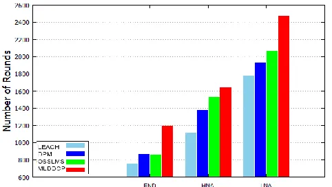
Protocol [6], Data Prediction Model for integrating WSN and Cloud (DPM) [11] and with Optimal Step Size Least Mean Square (OSSLMS) prediction algorithm[15]. The proposed algorithm is first compared with LEACH one of the most basic algorithms which provides clustering with the network. LEACH divides the sensing area into random clusters where the selection of CH is based upon probability analysis. The same approach has been used in the proposed protocol to elect CH in each round. Reason behind comparing the new protocol with LEACH is that it is most basic protocol which does not apply any data management technique. The results have been tabulated in following table 1, also simulation results have been given below. This algorithm outperforms from LEACH by a huge margin where FND performance is equivalent to HNA i.e. 50%. The LNA is also improved where MLDDCP has an edge of up to 700 messages from LEACH and other protocols. The designed protocol is compared with DPM and OSSLMS. When compared with DPM its FND is much ahead that of DPM. The similarity between DPM and MLDDCP is that both have a constant deterioration rate which means that nodes will not die instantly like in LEACH. The performance of LEACH is degraded in terms that there is a sharp steep moving from FND to HNA. But in case of DPM and MLDDCP this movement is fine and node die movement is gradual. When compared with OSSLMS algorithm this protocol still gives better results because the overhead with execution as well as processing time involved in OSSLMS algorithm makes it complex as compared to MLDDCP. Although performance of OSSLMS is better than LEACH and DPM but still there is a lack of no of nodes in contrast to MLDDCP. This algorithm outperforms from all the said protocols and the major reason for this is the selective movement of data. Where the last performance index of LEACH is near about 1700, DPM is 1900 and OSSLMS is 2000 the MLDDCP reaches near to 2500. This makes is more and more efficient. Another parameter that is compared and is measured with all four above mentioned protocols is throughput.
Table 1: Network Lifetime in terms of FND, HNA and LNA
Protocols FND HNA LNA
LEACH 755 1110 1780
DPM 870 1380 1930
OSSLMS 858 1530 2065
MLDDCP 1195 1640 2470
The experimental results show that in case of random environment when change of architecture is allowed and also the communication medium is unreliable i.e. the possibility of message to be lost during transmission is there. These assumptions have been introduced in the proposed algorithm to make it more resemblance to real situation. When this model feature is added to communication all the protocols behave differently where the performance of LEACH is drastically reduced, the DPM and OSSLMS algorithm shows stability towards the same. Again as dynamicity and unreliability is taken as an inherent feature of MLDDCP algorithm it gives better results in this environment.The throughput for LEACH is measured about 45%, and that of
DPM is 67%, OSSLMS is 73% and MLDDCP algorithm gives throughput of about 82%. LEACH has a low throughput value because of its lose control about message transmission. The message retransmission rate is very high in case of LEACH as no constraint has been applied on it. While DPM and OSSLMS have significantly high throughput value and the reason behind that is the check they apply in each round before transmission. MLDDCP algorithm has high throughput value and the reason is simple it measures the status of each message sent and retransmission is restricted by using a valid bit which when turned to 1 stops further retransmission for the current round.
Figure 2: Comparison of network lifetime of MLDDCP with OSSLMS, DPM and LEACH
Figure 3: Comparison of number of LIVE nodes per round
6 CONCLUSION
AND
FUTURE
SCOPE
5096 test the randomness of network and to trace out results every
time. It is therefore concluded that still in this random environment the proposed algorithm works very well and give better results.
It is clear from the results that selecting MLDDCP protocol will give a better result by reducing data traffic and increasing overall lifetime.
CONFLICT
OF
INTEREST
There is no conflict of interest.
REFERENCES
[1] I.F. Akyildiz, M.C. Vuran, “Wireless Sensor Networks”, John Wiley & Sons, 2010.
[2] Jain K, Bhola A (2018) Data Aggregation Design Goals for Monitoring Data in Wireless Sensor Networks. J Netw Secur Comput Networks 4:1–9.
[3] G. Wener-Allen, K. Lorincz, M. Ruiz, O. Marcillo, J. Johnson, J. Lees, M. Walsh, “Deploying a wireless sensor network on an active volcano, Data-Driven Applications in Sensor Networks”, IEEE Internet Computing, March/April 2006.
[4] Gupta K, Sikka V“Design (2015)Issues and Challenges in Wireless Sen-sor Networks” International Journal of Computer Applications 112(4):26-32, February.
[5] G. Anastasi, M. Conti, M. Di Francesco, and A. Passarella, “Energy conservation in wireless sensor networks: A survey”, Computer Networks (2009) pp. 537– 568.
[6] W.R. Heinzelman, A. Chandrakasan, H. Balakrishnan, “Energy-efficient communication protocol for wireless microsensor networks”, Proceedings of Hawaii International Conference on System Sciences (HICSS), January 2000, pp. 1–10.
[7] Jennifer Yick, Biswanath Mukherjee, Dipak Ghosal, “Wireless sensor network survey”, Computer Networks 52 (2008) 2292–2330.
[8] Subir Halder, Amrita Ghosal, “A survey on mobility-assisted localization techniques in wireless sensor networks”, Journal of Network and Computer Applications 60(2016)82–94.
[9] Gabriel Martins Dias, Boris Bellalta, And Simon Oechsner, “A Survey About Prediction-Based Data Reduction in Wireless Sensor Networks”, ACM Computing Surveys, Vol. 49, No. 3, Article 58, Nov 2016.
[10] Sotheara Say, Hikari Inata, Jiang Liu, and Shigeru Shimamoto, “Priority-Based Data Gathering Framework in UAV-Assisted Wireless Sensor Networks”, IEEE SENSORS JOURNAL, VOL. 16, NO. 14, JULY 15, 2016. [11] Samer Samarah, “Data Predication Model for Integrating
Wireless Sensor Networks and Cloud Computing”, Procedia Computer Science 52 (2015) 1141 – 1146. [12] Somasekhar Kandukuri, Jean Lebreton, Richard Lorion,
Nour Murad, and Jean Daniel Lan-Sun-Luk, “Energy-Efficient Data Aggregation Techniques for Exploiting Spatio-Temporal Correlations in Wireless Sensor Networks”, 2016 IEEE.
[13] Agarwal A, Gupta K, Yadav K. (2016) A Novel Energy Efficiency Protocol for Wsn Based on Optimal Chain Routing. IEEE Xplore 2016 3rd Int Conf Comput Sus-tain Glob Dev 488–493.
[14] D. Tulone, S. Madden, “Time series forecasting for approximate query answering in sensor networks”, Proceedings of the 3rd European Conference on Wireless Sensor Networks (EWSN), 2006, pp. 21–37.
[15] MouWu, Liansheng Tan, Naixue Xiong, “Data prediction, compression, and recovery in clustered wireless sensor networks for environmental monitoring applications”, Information Sciences 329 (2016) 800–818.
[16] Guiyi Wei , Yun Ling a, Binfeng Guo, Bin Xiao, Athanasios V. Vasilakos, “Prediction-based data aggregation in wireless sensor networks: Combining grey model and Kalman Filter”, Computer Communications 34 (2011) 793–802.
[17] L. Wang and A. Deshpande, “Predictive modeling-based data collection in wireless sensor networks”, Wireless Sensor Networks, pp. 34–51, Springer, 2008.
[18] Reicherdt R., Glesner S. (2014) Formal Verification of Discrete-Time MATLAB/Simulink Models Using Boogie. In: Giannakopoulou D., Salaün G. (eds) Software Engineering and Formal Methods. SEFM 2014. Lecture Notes in Computer Science, vol 8702. Springer, Cham. [19] Guo, W., Xiong, N., Vasilakos, A. V., Chen, G., & Cheng,
H: Multi-source temporal data aggregation in wireless sensor networks, In: Wireless Personal Communications, (2011), 56, 359–370.
[20] H. Jiang, S. Jin, C. Wang: Prediction or not? An energy-efficient framework for clustering-based data collection in wireless sensor networks, In: IEEE Trans.Parallel Distrib. Syst. 22 (6) (2011) 1064–1071.