Contents lists available atScienceDirect
Physica Medica
journal homepage:www.elsevier.com/locate/ejmp
Original paper
In-vivo EPID dosimetry for IMRT and VMAT based on through-air predicted
portal dose algorithm
M.A. Najem
a,⁎, M. Tedder
b, D. King
a, D. Bernstein
a, R. Trouncer
a, C. Meehan
a, A.M. Bidmead
aaJoint Department of Physics, The Royal Marsden NHS Foundation Trust and The Institute of Cancer Research, Fulham Road, London SW3 6JJ, UK bMedical Physics Department, Guy’s and St Thomas’NHS Foundation Trust, London SE1 7EH, UK
A B S T R A C T
We have adapted the methodology of Berry et al. (2012) for Intensity Modulated Radiotherapy (IMRT) and Volumetric Modulated Arc Therapy (VMAT) treatments at afixed source to imager distance (SID) based on the manufacturer’s through-air portal dose image prediction algorithm. In order tofix the SID a correction factor was introduced to account for the change in air gap between patient and imager. Commissioning data, collected with multiplefield sizes, solid water thicknesses and air gaps, were acquired at 150 cm SID on the Varian aS1200 EPID. The method was verified using six IMRT and seven VMAT plans on up to three different phantoms. The method’s sensitivity and accuracy were investigated by introducing errors. A global 3%/3 mm gamma was used to assess the differences between the predicted and measured portal dose images. The effect of a varying air gap on EPID signal was found to be significant–varying by up to 30% withfield size, phantom thickness, and air gap. All IMRT plans passed the 3%/3 mm gamma criteria by more than 95% on the three phantoms. 23 of 24 arcs from the VMAT plans passed the 3%/3 mm gamma criteria by more than 95%. This method was found to be sensitive to a range of potential errors. The presented approach provides fast and accurate in-vivo EPID dosimetry for IMRT and VMAT treatments and can potentially replace many pre-treatment verifications.
1. Introduction
Intensity Modulated Radiotherapy (IMRT) and Volumetric Modulated Arc Therapy (VMAT) enable the delivery of highly con-formal and uniform dose distributions to planning target volume (PTV) whilst sparing organs at risk (OARs)[1]. While this enhanced delivery capability has been shown to be advantageous with respect to im-proving patient outcome[2,3], it does introduce new challenges for the quality assurance (QA) of treatments in term of additional linac QA as well as patient-specific QA, which is recommended to be carried out prior to, or within the first few fractions of treatment [4,5]. In vivo dosimetry is a form of patient-specific QA that offers certain advantages over pre-treatment QA, namely that it actually verifies what is really of interest: the dose delivered to the patient. Within 4 years at the Neth-erland Institute of Cancer Research, more than 4000 plans were verified using an in-vivo dosimetry system. Of the 17 serious errors detected, 9 would not have been detected with pre-treatment verification[6]. The same conclusion was obtained from another study by the same institute carried out on more than 15,000 plans. 35 serious errors were detected that would not have been detected with pre-treatment verification due to mainly changes in patients anatomy[7].
EPID dosimetry can offer advantages in terms of the ease and speed with which in vivo dosimetry can be performed, the extra information afforded by sampling the entire radiationfield rather than just a single
point (as by using thermo-luminescent detectors (TLDs) or diodes), and the additional scope it offers for detecting changes in patient anatomy [8–10]. EPID dosimetry can be performed in many different ways, an overview of which is given in the literature review by Van Elmpt et al. [11]. Within the subcategory of in vivo EPID dosimetry several im-plementations have been developed each of which verifies the dose to the patient in different ways. Several in-vivo EPID software solutions have been commercially available recently and have been assessed in a number of studies[12,13]. However, the solutions thus far have mainly been developed in house by academic centres, resulting in a wide variety of methodologies. These methodologies can be divided into: a point dose verification in the patient, 2D transit dose verification at the level of the EPID, 2D transit dose verification in a plane in the patient or 3D transit dose verification in the patient [14–19]. A recent study by Bedford et al. (2017) investigated the agreement between the forward and back-projection transit EPID dosimetry for prostate radiotherapy. They found a fairly similar response from both methods and they concluded that both of them can be used to verify the dose delivered to the patient[20].
Van Elmpt et al. (2005) developed a system that predicted a transit portal dose image using a through air portal dose image and the radi-ological thickness of the path of the beam through the patient[21].
Berry et al. (2012) used a similar technique, but rather than using a measured through air portal dose image, they used the image predicted
https://doi.org/10.1016/j.ejmp.2018.07.010
Received 19 April 2018; Received in revised form 2 July 2018; Accepted 24 July 2018
⁎Corresponding author.
E-mail address:[email protected](M.A. Najem).
Available online 02 August 2018
1120-1797/ © 2018 Associazione Italiana di Fisica Medica. Published by Elsevier Ltd. This is an open access article under the CC BY-NC-ND license (http://creativecommons.org/licenses/BY-NC-ND/4.0/).
by the Varian Portal Dosimetry software, which is based on the work of Van Esch et al. [15,22]. However, in their model, a fixed air gap of 35 cm was used between the phantom exit and EPID. Thefixed air gap causes several problems. Firstly, it increases the treatment time for each patient as the EPID needs to be moved for each beam in order to keep a constant air gap which has several consequences including increased risk of intra-fraction motions and reduced patient throughput. Sec-ondly, it increases the generation time of the portal dose images through air since each beam requires a verification plan with a different source to imager distance (SID) to be created in the Eclipse treatment planning system (TPS). Finally, it is not suitable for VMAT treatments as EPID needs to be at afixed SID while the gantry rotates. Another lim-itation of the original methodology used by Berry et al. was that they did not include the couch model in their calculations, and consequently reported a decrease in the mean gamma pass rate forfields that transit the couch[23].
The aim of this work is to extend the methodology of Berry et al. (2012) to be used for both IMRT with afixed SID and VMAT treatments. This is achieved by introducing a correction factor which takes into account the change in air gap between the patient exit and EPID for a fixed SID. To improve the accuracy of the system, the couch model was included in our calculation to take into account the couch attenuation at any gantry angle. In addition, a new approach to calculate IMRT and VMAT equivalent squarefield size is presented.
2. Materials and methods
2.1. Equipment
Portal dose images were delivered on a Varian TrueBeam linac which is equipped with the Varian portal imager aS1200. This imager has a sensitive area covering a 40 × 40 cm2field size at a 100 cm SID and high resolution (1190 × 1190 pixels) in the dosimetry mode. In addition, it has a backscatter shield to remove the effect of uneven backscatter from the support arm [24]. Portal dose images were ac-quired at dose rate up to 600 MU/min (the max dose rate for 6 MV beam) on this machine.
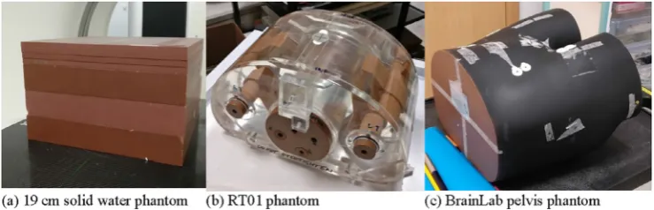
The imager was calibrated according to the manufacturer's re-commendation and the central pixel value calibrated to equal 0.444 CU (calibrated unit) when irradiated with 100 MU and a 10 × 10 cm2field at 150 cm SID. All measured portal dose images (mIs) in our experi-ments were acquired at a 150 cm SID. Three phantoms were used in the verification: A 30 × 30 × 19 cm3water-equivalent“solid water (SW)” phantom, the RT01 phantom and the BrainLab pelvis phantom (BrainLab Medical Systems, Westchester, IL) (seeFig. 1) [25]. In ad-dition, slabs of tissue-equivalent materials (water, bone and lung) were used to create phantoms with a range of complexities in order to test the accuracy of the presented model.
The predicted portal dose images through air (pIsair) were created using Eclipse v13.7. For an in-depth description of howpIsairare cal-culated, see the paper by Van Esch et al. [22]. The RT plan, RT
structure, CT images and pIsair are imported to in-house software written in Python v3.5.1 in order to calculate the predicted images through patient (pIsp).
2.2. Predicted images through patient model
ThepIpfor anyfield size (FS), thickness (t), air gap (g) andfixed SID can be calculated from thepIsairat any position (x, y) on the EPID using the following equation:
= ∙ ∙ ∙
pIp pIair T x y FS t( , , , ) OAR x y t( , , ) G x y FS t g( , , , , ) (1) Each of the terms in Eq.(1)is briefly described inTable 1below.
2.2.1. Transmission correction factor model
In the implementation used by Berry et al. (2012), two terms were used to account for the two primary causes of attenuation of the beam through the phantom: the attenuation of the primary beam, which was modelled in narrow beam conditions using Monte Carlo (MC) simula-tions, and the effect of scattered and secondary radiation, which was empirically derived by measuring the EPID response for severalfield sizes and SW block thicknesses [15]. In this work, both terms are combined into one empirically derived correction factor dependent on attenuator thickness andfield size. A series of images were acquired with the EPID for differentfield sizes and thicknesses of SW blocks to determine the equation that defines this correction factor. The data werefitted using a nonlinear least squares method to the following equation:
= +
− −
T t FS A FS e C FS e
S FS
( , ) ( ) ( )
(0, )
B FS t( ) D FS t( )
(2) where A FS( )=a e−a FS+a
1 2 3, B FS( )=b FS1 b2, C FS( )=c e1 −c FS2 +c3, =
D FS( ) d1FSd2.
S(0,FS)is the mean signal in the 4 × 4 pixels at the EPID centre produced by the beam with no attenuation for a given field size.
a a a b b1, 2, 3, 1, 2,c c c d d1, 2, 3, 1, 2are empirically determinedfitting para-meters. Table 2 summarises the commissioning measurements per-formed to determine the T factor. The model was then verified with a mix offield sizes and SW thicknesses.
Fig. 1.Phantoms used to verify our method: (a) a 19 cm solid water phantom, (b) the RT01 phantom and (c) the BrainLab pelvis phantom. Table 1
A brief summary of each term in Eq.(1).
Parameter Description
T Transmission factor which takes into account the attenuation of the beam through the phantom
OAR The off-axis pixel response function, that accounts for the fact that the offaxis spectrum of the incident beam varies as a function of radial distance from the central axis
2.2.2. Off-axis pixel response factor model
This correction factor is derived empirically, using a similar set of data as for the T correction factor, but with only afield size that fully covers the EPID at 150 cm SID (27 × 27 cm2). A third-degree poly-nomial is used to fit the OAR factor for each individual pixel as a function of the attenuator thickness as described in the following equation:
= + + +
OAR i j( , ) α i j t i j1( , ) ( , )3 α i j t i j2( , ) ( , )2 α i j t i j3( , ) ( , ) α i j4( , )
(3) For a given pixel at the ith row and jth column
α i j1( , ),α i j2( , ),α i j3( , ),α i j4( , ) are empirically determined fitting parameters andt i j( , )is the equivalent radiological path length traced through the CT scan to the pixel.
Table 3summarises the commissioning measurements performed to determine the OAR factor.
2.2.3. Air gap correction factor model
A series of portal dose images were acquired with the EPID for differentfield sizes, thicknesses of SW blocks and air gaps to determine the correct model for this factor. In this work, the G factor is divided into two terms:
=
G x y t FS g( , , , , ) G t FS g G x y gc( , , ) o( , , ) (4)
whereG t FS gc( , , )is the air gap factor at the centre region (the 4 × 4 pixels at EPID centre) of the EPID which is a function of thickness,field size and air gap.G x y go( , , )is the air gap off-axis pixel response function which takes into account the change in off-axis pixel response due to the change in air gap distance. Both factors were normalised to a 40 cm air gap. A multi-dimensional look-up table to interpolate betweenfield sizes, thicknesses, and air gaps is used to model theGc factor. TheGo factor wasfitted using a nonlinear least squares method to the following equation:
= −
G x y go( , , ) e Δ( ).Ω( , )g x y (5)
where:Δ( )g =β g g1( −0)2+β g g( − )+β
2 0 3, =
+ x y
Ω( , ) γ x y γ
( )
1 2 2
2 .
where β β1, 2,β γ γ3, 1, 2are the empirically determined fitting para-meters andg0is the default air gap at which the other correction factors were modelled. In this work,g0=40cm.Table 4summarises the com-missioning measurements used to determine the G factor.
2.2.4. The equivalent thickness map
In order to predict the effect of patient (phantom) attenuation on pIair, information about the radiological path length for each photon beam arriving at the EPID is required. The patient CT scan is used along with a calibration table which converts from Hounsfield Units (HU) to electron density to calculate electron density at each voxel in the CT scan. The body outline from the structure set is used to restrict the
calculated voxels to just those within the body. The couch structure, generated in the Eclipse TPS, is also included in the calculation so that the attenuation through the couch at any gantry angle is included. The radiological path length is then calculated for each ray arriving at a pixel at the EPID using the method reported by Siddon[26]. The ray tracing algorithm was verified using virtual phantoms with known geometries and densities as well as comparing the equivalent thickness at the central axis for each verification plan to that obtained from Eclipse TPS. The calculated equivalent thicknesses were found to agree with those calculated in Eclipse to within ± 1 mm.
2.2.5. Equivalent squarefield size for dynamicfields
To assess the impact of both the collimator and MLC positions on the estimation of the equivalent squarefield size, we investigated if the equivalent squarefield size for a given dynamicfield can be calculated from only thefield formed by X and Y secondary collimators. Several dynamic fields with the same X and Y secondary collimator (i.e. 10 × 10 cm2) opening but different fluence map were delivered through a 20 cm thick SW phantom at three different air gaps: 20, 30 and 40 cm.Fig. 2shows thefluence map for each dynamicfield. It was found that the correction factors depend on both totalfluence and open area and not only on the X and Y collimator size. The equivalent square field sizeFS, which gives the best agreement with our measurements, was found to be calculated using the following empirical equation:
=
FS FS A
A
OF f
OF (6)
whereFSOFis the equivalent squarefield size calculated from X and Y collimators,Af is the area in thefield where thefluence is larger than zero, andAOFis the area within thefield formed by X and Y collimators.
2.3. Predicted images through patient model verification
Six IMRT plans and seven VMAT plans were used to verify the presented method. The IMRT plans were clinical prostate and seminal vesicle plans; two were planned according to the CHHiP trial protocol, two to the PACE protocol, and two according to the pre-CHHiP clinical standard at RMH[27,28]. The VMAT plans consisted of prostate bed (n = 2), prostate and nodes (n = 2), larynx bed (n = 2), and vagina (n = 1) plans. Each plan was delivered on up to three different phan-toms described inSection 2.1. In total, 15 IMRTfields were delivered to the RT01 phantom, 15 IMRTfields and 12 VMAT arcs were delivered to the 19 cm solid water phantom, and 30 IMRTfields and 12 VMAT arcs were delivered to the BrainLab pelvis phantom. pIsp and mIs were compared using a global 3%/3 mm gamma evaluation with 10% dose threshold as it is the most common gamma criteria used in dosimetric QA[29].
In addition,pIsp andmIs were compared using a local 2%/2 mm Gamma criteria to test the sensitivity of the system[29].
All plans used were independently verified using PTW OCTAVIUS 1500 ionisation chamber array (PTW, Freiburg, Germany) and/or Varian pre-treatment verification (Portal Dosimetry) software. All plans passed the local 3%/3 mm gamma evaluation by more than 98% on the PTW array and by more than 99% on Varian pre-treatment verification Table 2
The commissioning measurements used to model the T factor.
Field size (cm2) Solid water thickness (cm) Air gap (cm) Gantry (deg) MUs
3 × 3, 5 × 5, 8 × 8, 10 × 10, 15 × 15, 20 × 20, 25 × 25
0, 5, 10, 15, 20, 25, 30, 35, 40
40 270 100
Table 3
The commissioning measurements used to model the OAR factor.
Field size (cm2) Slabs thickness (cm) Air Gap (cm)
Gantry (deg) Mus
27 × 27 0, 1, 2, 3, 5, 10, 15, 20, 25, 30, 35, 40
40 0 100
Table 4
The acquisition parameters used to model the G factor.
Field size (cm2) Slabs thickness (cm)
Air gap (cm) Gantry (deg)
MUs
5 × 5, 10 × 10, 15 × 15, 20 × 20
0, 10, 15, 20, 25, 30, 35, 40
20, 25, 30, 35, 40, (45, 50, 55)*
0 100
software.
2.3.1. The effect of heterogeneity
To investigate the ability of our model to predict accurate portal dose images in the presence of heterogeneities, an anterior IMRTfield from one of the six prostate plans was delivered on several phantoms
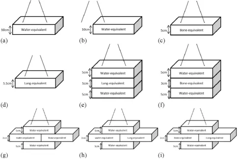
(shown in Fig. 3). These phantoms were made of tissue-equivalent materials; water (WT1, relative electron density = 1.0), cortical bone (SB5, relative electron density = 1.73) and lung (LN10, relative elec-tron density = 0.3)[30]with a range of complexities similar to what was presented by the work of Berry et al.[15].
The following geometries and material configurations were Fig. 2.Thefluence maps used to determine the equivalent squarefield size for a dynamicfield.
measured with the field pointing directly at the phantom: single ma-terials (Fig. 3a–d), single material with a beam passing through part of the phantom only (Fig. 3b), multiple materials with tissue boundaries along the ray path (Fig. 3b–f), multiple materials with tissue boundaries both along the ray path and perpendicular to the treatment field (Fig. 3g–i)
2.4. Model sensitivity
2.4.1. Error detection
In order to test the sensitivity of our model to detect dose delivery errors in the patient, several types of errors were deliberately in-troduced either into the plan itself or the phantom setup. This was done using a single IMRT verification plan and followed an approach similar to that of Bedford et al.[14]. ThepIspfor the unaltered plan and setup were compared to themIsfor the delivery containing the errors, to test whether the dose discrepancy is greater than that observed for the unaltered IMRT plan and therefore determine whether the error can actually be detected.
The deliberate errors were all introduced to a prostate IMRT plan, created in accordance with the CHHiP trial protocol. The error plans were all delivered to the BrainLab pelvis phantom apart from in the case of the change in phantom size, which was done using SW blocks. The errors introduced were:
1. Dose errors: The number of monitor units for allfields in the plan was altered by−5%, +1%, +3%, +5% and +10%, creatingfive new plans with deliberate errors in. All other aspects of the plan were kept the same.
2. Gantry angle error: Two plans were created, identical to the original plan on the BrainLab pelvis phantom, except with gantry angle offsets of +5° and +10° introduced.
3. Patient set-up errors: One field from the original plan (the left anterior obliquefield, at a gantry angle of 35°) was delivered to the BrainLab pelvis phantom, but with the phantom offset by 0.5 cm, 1 cm, 1.5 cm and 2 cm laterally towards the patient’s right, and by the same offsets in the anterior direction, resulting in 8 deliveries of onefield.
4. Change in phantom size: For this sensitivity test, the posteriorfield (180°) from the original plan was delivered to the CT scanned 19 cm solid water block, with 0.5 cm, 1 cm, 2 cm and 3 cm of solid water added on top; only the posteriorfield was measured to save time, as this was thefield that would be most affected by a change in depth of the phantom.
5. MLC errors: new versions of the original plan were created with MLC errors introduced by altering the MLC planfile using a python script. The MLCfiles were then imported back into Eclipse, and the plan was calculated again using the new MLC positions. The type of MLC errors and thefields which they were applied to is detailed in
Table 5.
3. Results
3.1. Transmission correction factor
The T factor wasfitted successfully using Eq.(2). The R2value of the fitted equation was found to be 0.9998. Thefitting parameters are listed in Table 6. Fig. 4 shows the measured and modelled T factor as a function of SW thickness for severalfield sizes. A comparison of the measured and modelled T factors for severalfield sizes and SW thick-nesses is shown onTable 7.
3.2. Off-axis pixel response factor
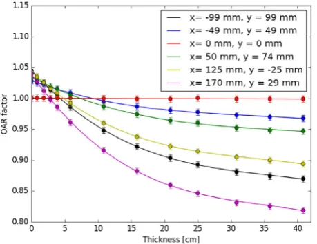
All measured and modelled OAR model images passed the 0.5%/ 0.5 mm 2D gamma by 100%.Fig. 5shows the measured and modelled OAR factors as a function of SW thickness at different positions on the EPID.
3.3. Air gap correction factor
Fig. 6a shows the measured and modelled Gc factors for a 15 × 15 cm2field size as a function of SW thickness at different air gaps. Fig. 6b shows Gc factor for 30 cm solid water thickness as a function offield size for different air gaps.
A comparison of the measured and modelledGcfactors for several field sizes, SW thicknesses and air gaps is shown inTable 8.
Table 5
The MLC errors that were deliberately introduced into eachfield of one of IMRT plans in order to test the sensitivity of portal dosimetry to different types of MLC error.
Error Field (Gantry angle [deg])
MLC error
E1 Allfields Both banks shifted in the same direction by 5 mm E2 POST (180°) Shift both leaf banks in by 2 mm
E3 LPO (100°) Shift the leaves of bank B that are within thefield in by 5 mm
E4 LAO (35°) Shift one leaf in bank A that is close to the centre of thefield in by 1 cm
E5 RAO (325°) Open all leaf pairs that are within thefield out by 5 mm
E6 RPO (260°) Shift four leaves from bank A at the superior edge of the treatmentfield by 1 cm
Table 6
T factorfitting parameters.
= −
a1 0.9580 a2=0.0185 a3=0.9529 b1=0.4143 b2= −0.7029 = −
c1 50.2717 c2= −0.0002 c3=50.6647 d1=0.0548 d2= −0.1675
Fig. 4.The measured (circles) and modelled (lines) T factors as a function of solid water thicknesses for differentfield sizes.
Table 7
The modelled and measured T factors for differentfield sizes and SW thick-nesses.
Field Size (cm) Thickness (cm) Measured (CU) Modelled (CU) Diff(%)
25 × 25 2.84 0.419 0.4191 0.0
7 × 18 17 0.187 0.1865 −0.3
13 × 13 17 0.197 0.1968 −0.1
7 × 14 23.84 0.134 0.1337 −0.2
Fig. 7a and b show theGofactor along the x-axis at 30 cm air gap for a 15 × 15 cm2field size and different SW thicknesses and 20 cm solid water thickness and differentfield sizes, respectively.Fig. 7c shows the measured and modelledGofactor along the x-axis as a function of air gap for a 20 × 20 cm2field size and 20 cm SW thickness.Fig. 7d shows the difference between the modelled and measuredGofactor for different air gaps.Table 9lists thefitting parameters used tofit Eq.(5). The R2 value of thefitted equation was found to be 0.9994.
3.4. Verification results
3.4.1. IMRT plans
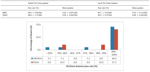
All IMRT fields (60 fields in total) passed the 3%/3 mm gamma criteria by more than 95%. The average gamma pass rate was 99.8 ± 0.3(1SD), 99.9 ± 0.3(1SD) and 99.3 ± 1.2(1SD) for 19 cm SW, RT01 and BrainLab pelvis phantoms, respectively.Fig. 8shows a histogram of gamma pass rate for all IMRT fields on the three phan-toms. The average gamma pass rate for beams which do and do not pass through the couch was found to be the same (99.6 ± 0.9(1SD)). 45 of 60fields passed the local 2%/2 mm gamma criteria by more than 95%. The overall global 3%/3 mm and local 2%/2 mm gamma pass rate and mean gamma for all IMRTfields are listed inTable 10.
3.4.2. VMAT plans
For VMAT plans, 23 of the 24 arcs passed the 3%/3 mm gamma
criteria by more than 95%. However, the 3%/3 mm gamma pass rate of the failed arc was 94.6%. The mean 3%/3 mm gamma pass rate was 98.7 ± 1.8(1SD) and 98.9 ± 1.5(1SD) for the 19 cm SW and BrainLab pelvis phantoms, respectively.Fig. 9shows a histogram of gamma pass rate for all VMATfields on the 19 cm SW and BrainLab pelvis phantoms. None of the VMAT plans passed the local 2%/2 mm gamma criteria by more than 95%. The overall global 3%/3 mm and local 2%/2 mm gamma pass rate and mean gamma for all VMAT arcs are listed in Table 10.Fig. 10shows thepIpandmIsimages and global 3%/3 mm and local 2%/2 mm gamma maps for a VMAT field delivered on the BrainLab pelvis phantom.
3.4.3. The effect of heterogeneity
All beams, delivered on phantoms shown inFig. 3, passed the 3%/ 3 mm gamma criteria by more than 99.5% (see Fig. 1 in the Supplementary material).
3.5. Model sensitivity
3.5.1. Error detection
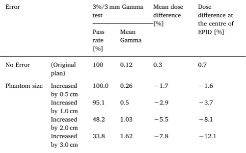
Table 11shows the 3%/3 mm gamma pass rate for the plans with errors deliberately introduced that were delivered on the BrainLab pelvis phantom.
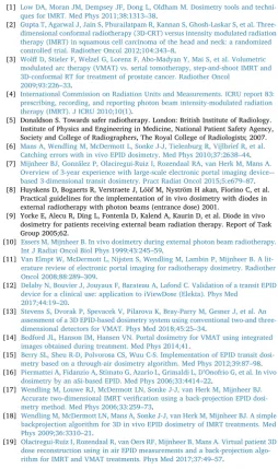
Table 12shows the 3%/3 mm gamma pass rate and mean gamma, mean dose difference and the dose difference at the centre of the EPID between the measured and predicted images for errors plans delivered on a 19 cm SW phantom.
4. Discussion
As can be seen in Fig. 4, the modelled T factor was in a good agreement with measured values. The difference between the measured and modelled T factor for differentfield sizes and SW thicknesses was Fig. 5.The measured (circle) and modelled (line) OAR factors as a function of
solid water thicknesses at different locations on the EPID. Note the error bars illustrate a 0.5% difference in OAR value at each point.
Fig. 6.The measured (circle) and modelled (line)Gcfactor at different air gaps as (a) a function of attenuator thickness for a 15 × 15 cm2field size and (b) as a function offield size for a 30 cm solid water thickness.
Table 8
The modelled and measured Gcfactors for differentfield sizes, SW thicknesses and air gaps.
FS (cm2) t (cm) g (cm) Measured Modelled Diff(%)
13 20.84 35 1.024 1.024 0.0
13 20.84 30 1.054 1.052 −0.2
13 20.84 20 1.151 1.149 −0.1
13 20.84 37 1.012 1.014 0.2
7.9 30.46 35 1.019 1.013 −0.6
7.9 30.46 30 1.029 1.032 0.4
10 9.34 35 1.011 1.010 −0.1
found to be less than 0.5% as seenTable 7. Berry et al. (2012) used two terms to model this factor and carried out several MC simulations to calculate the mass attenuation factor for a 6 MV photon beam[15].
However, we found that using one term to model this factor was suf-ficient and easier to implement since no MC simulations are required.
With regards to OAR factor, the third-degree polynomial model at each individual pixel was found to accuratelyfit this factor (Fig. 5). All commissioning images passed by 100% the 0.5%/0.5 mm 2D gamma evaluation. The third-degree degree polynomial model was found to give better agreement in our work compared with the Gaussian model introduced by Berry et al. (2012). This difference could be due to the Fig. 7.The measuredGofactor at a 30 cm air gap for (a) a 15 × 15 cm2field size and different thickness and (b) for a 20 cm solid water thickness and differentfield sizes. (c) The measured (dashed line) and modelled (solid line)Gofactor along the x-axis for a 20 × 20 cm2field size, 20 cm SW thickness and several air gaps. (d) The percentage difference between the measured and modelledGofactor along the x-axis for different air gaps.
Table 9
Thefitting parameters ofGofactor.
= −
β1 7.5902 108 β2=1.0211 β3=40.1247 γ1= −28.6866 γ2=26.7742
< 95% 95% -96% 96% - 97% 97% - 98% 98% - 99% 99% - 100%
RT01 0 0 0 0 6.7 93.3
SW19cm 0 0 0 0 6.7 93.3
Pelvis 0 3.3 3.3 3.3 16.7 73.4
0 25 50 75 100
Per
centage of
beams
(%)
3%/3mm Gamma pass rate (%)
Table 10
The overall global 3%/3 mm and local 2%/2 mm gamma pass rate and mean gamma for all IMRT and VMAT plans.
Global 3%/3 mm gamma Local 2%/2 mm Gamma
Pass rate [%] Mean gamma Pass rate [%] Mean gamma
IMRT 99.6 ± 0.9(1SD) 0.22 ± 0.07(1SD) 96.1 ± 5.5(1SD) 0.33 ± 0.11(1SD)
VMAT 98.8 ± 1.7(1SD) 0.30 ± 0.05(1SD) 84.5 ± 6.7(1SD) 0.82 ± 0.32(1SD)
< 95% 95% -96% 96% - 97% 97% - 98% 98% - 99% 99%
-100%
SW19cm 7.1 7.1 0.0 7.1 0.0 64.3
Pelvis 0.0 14.3 0.0 0.0 14.3 57.1
0.0 35.0 70.0
Per
centage of beam
s
(%
)
3%/3mm Gamma pass rate (%)
Fig. 9.3%/3 mm gamma pass rate histogram for VMATfields delivered on the 19 cm SW and BrainLab phantoms.
EPID model (aS1000) that they used in their study. In addition, Berry et al. used a field size specific backscatter correction that was pre-viously developed for portal dosimetry by the same group[31]. In this work, no backscatter correction was used with the aS1200 since this EPID model has backscatter shield to remove the effect of uneven backscatter from the support arm[24].
It can be found fromFig. 6a and b that the effect of air gap is not negligible and the EPID signal can vary by up to 30% for the smallest air gap and largestfield size and SW thickness. TheGcfactor was found to increase as the field size and thickness increases and as the air gap decreases. This could be due to the increase in secondary (scattered) photons that reach the EPID. We used a multi-dimensional look-up table to calculate theGcfactor for a givenfield size, attenuator thickness and air gap as nofitting equation was found to model this factor ac-curately. The difference between the measured and calculated values for several images with a range offield sizes, SW thicknesses and air gaps was found to be less than 1% as seen inTable 8.
As seen inFig. 7a–c, theGofactor is relatively independent offield
size and thickness, and is only affected by distance between the patient exit and EPID. Eq.(5)was found to accurately model this factor with R2 equal to 0.9994 as can be seen inFig. 7c. The difference between the measured and modelled factor was found to be less than 1% at any point as seen inFig. 7d.
Even though the effect of air gap on EPID central axis dose was studied by Talamonti et al. (2006) for pre-treatment IMRT verification [32], to the authors' knowledge, no one has introduced a model to correct the EPID in-axis and off-axis pixel response due to the change in the air gap between the patient and the imager.
The introduced model verified successfully for several IMRT and RA plans on up to three different phantoms. Most IMRT and RA fields passed the 3%/3 mm gamma criteria by more than 99% as can be seen in Figs. 8 and 9which is similar or superior to results published in previous studies[14,15,33].
Berry et al. (2014) evaluated their model on 11 patients. They found that the average 5%/3 mm gamma pass rate was increased from 89.1% to 95.7% by excluding all beams that interfere with the couch[23]. Since the couch structure was included in our model, no difference was noticed in gamma pass rate between beams that interfere and do not interfere with the couch. Therefore, the evaluation of the portal dose images in our model should not be influenced by beams transmission through the couch.
In order to determine the specificity and sensitivity of the system we both introduced deliberate errors and varied the gamma criteria. The high failure rate with a 2%/2 mm gamma criteria (seeSections 3.4.1 and3.4.2), when no deliberate errors were presented, means that the specificity at this gamma criteria is too low for the system to be clini-cally useful. At 3%/3 mm, the specificity is sufficient for the test to be useable. The sensitivity at this level is discussed below. The low spe-cificity of the system at 2% 2 mm gamma may be due to our not ac-counting for higher-order scattering components[34]. In addition, the effect of penumbra and inter-leaf leakage is more pronounced in the highly modulated treatments such as VMAT treatments[35]. It may be possible to improve the accuracy of the system by taking further mea-surements in order to produce a scatter kernel that, when convolved with the predicted image, will improve agreement with measurements. However, the 3% 3 mm gamma criteria used compares favourably to other published work. For example, Bedford et al. (2014) reported an average 3%/3 mm global gamma pass rate from 9 VMAT plans equals to 93.7 ± 3.0[14]. In addition, the 3%/3 mm gamma pass rate in our method is considerably more than the action level of 90% per treatment field that was recommended in AAPM TG-119 for pre-treatment ver-ification [36]. The differing patterns of failure for different beams shown inTable 11, discussed in more detail below, demonstrates that the failures are not due to systematic high or low predictions.
The predicted portal dose images for IMRTfields through different heterogeneous phantoms can be calculated accurately by our method, achieving 3%/3 mm gamma pass rate of more than 99.5% on all the phantoms tested, as shown inFig. 3. The geometries were simple, but featured large discontinuities and materials with different electron densities. Diagram b inFig. 3indicates that the presented method could be used for treatments where part of thefield extends beyond the pa-tient (e.g. breast treatments).
From the results reported in Table 11, the introduced method should be sensitive to dosimetric errors, the level of which is dependent on the gamma criteria used. The higher the dose criteria, the less sen-sitive the method will be to dose errors, as expected. Increasing the MUs by more than 3% caused allfields to have passing rates at 3%/3 mm gamma criteria of less than 95%. These results agreed with the results reported by Bedford et al. (2014) as all plans in their study fail the gamma evaluation when they increase the number of MUs by 10%[14]. The results inTable 11demonstrate that in principle, our method should be sensitive to gantry angle errors, as the passing rates for some of thefields delivered in the prostate plans, for both 5° and 10° shifts, change markedly. For smaller angular rotations it is less likely to cause Table 11
The 3%/3 mm gamma pass rate for the error plans (seeSection 2.4.1) that were delivered on the BrainLab pelvis phantom.
Error 3%/3 mm Gamma pass rate [%]
POST LPO LAO RAO RPO
No error (original plan) 99.9 98.2 100.0 99.9 98.1 Dose MUs increased by 1% 97.9 97.9 99.6 99.3 97.7 MUs increased by 3% 79.8 82.6 94.9 95.5 93.6 MUs increased by 5% 62.5 59.5 79.0 76.5 73.3 MUs increased by 10% 44.3 48.7 55.3 53.2 51.5 MUs decreased by 5% 97.9. 94.7 83.1 71.3 84.0
Gantry angle Offset by +5° 97.8 99.0 94.1 91.3 98.6
Offset by +10° 98.1 94.7 79.6 68.8 97.8
Set-up error Offset by 0.5 cm (right) 100.0
Offset by 1.0 cm (right) 100.0
Offset by 1.5 cm (right) 99.7
Offset by 2.0 cm (right) 97.8
Offset by 0.5 cm (ant) 100.0
Offset by 1.0 cm (ant) 100.0
Offset by 1.5 cm (ant) 99.9
Offset by 2.0 cm (ant) 99.6
MLC E1,Table 5(not aligned) 61.3 51.4 46.4 62.8 59.0 E2,Table 5 79.5
E3,Table 5 47.9
E4,Table 5 98.3
E5,Table 5 14.5
E6,Table 5 94.3
Table 12
The gamma pass rate and mean gamma at 3%/3 mm, mean dose difference and the dose difference at the centre of the EPID between the measured and pre-dicted images for errors plans delivered on a 19 cm SW phantom.
Error 3%/3 mm Gamma
test Mean dose difference [%] Dose difference at the centre of EPID [%] Pass rate [%] Mean Gamma
No Error (Original plan)
100 0.12 0.3 0.7
Phantom size Increased by 0.5 cm
100.0 0.26 −1.7 −1.6
Increased by 1.0 cm
95.1 0.5 −2.9 −3.7
Increased by 2.0 cm
48.2 1.03 −5.5 −8.1
Increased by 3.0 cm
a noticeable drop in passing rates, as the smaller the rotation from the planned position the difference in the geometry that the beam transits. The precise level of gantry error that will be detected will depend on several factors including the specific patient anatomy and the location of fields with respect to the anatomy. This shows that our method should provide a way of detecting such an error, if a significant one were to occur.
The reported results fromTable 11show that, as might be expected, set-up errors of up to 2 cm shifts of the patient in one direction do not result in passing rates that would indicate that an error has occurred. This result agrees with the results reported by Bedford et al.[14]. While these set-up errors would result in significant errors for the patient in terms of dose localisation, the differences in the measured portal dose images are small because the anatomy that the beam passes through, for a prostatefield shifted by 2 cm relative to the patient, does not change drastically. The sensitivity of the system to geometrical shifts will de-pend on the anatomy of the patient, for example, the presence of sig-nificant inhomogeneities in and around the treatment field, where greater inhomogeneity increases the likelihood of detecting positional errors. Our model was not intended to detect such set-up errors how-ever, therefore the current protocols for treatment that are in place to produce the correct set-up of the patient, such as kV imaging, should be maintained in order to ensure this.
The results of the verification measurements performed on plans containing deliberate MLC errors, described inTable 11, demonstrate that the current method is sensitive to a range of MLC errors. This is consistent with the results reported by Bedford et al.[14]. The varied MLC errors introduced to the individualfields (E2 to E6 inTable 5) all produced distinct features in the gamma maps, making our model sensitive to these errors. However, the MLC errors introduced are un-likely to occur during treatment and more subtle MLC errors may not be detected by the presented model at all.
Table 12reports the results of thefield verification measurements performed with additional slabs of solid water added to the solid water slab phantom to simulate changes to the patient outline: they demon-strate that a change in water equivalent path length of 1 cm for an original path length of roughly 20 cm should be detectable for IVED. This type of error was not included in the study by Bedford et al.[14]. The precise thickness change that will result in a significant drop in the gamma passing rate will depend on the gamma criteria used, and the original path length of the beam through the patient; the larger the patient, the less changes in equivalent thickness will affect the mea-sured dose at the EPID. Although the gamma pass rate did not drop enough to indicate an error for an additional 1 cm of SW, the error could be indicated via changes in the mean gamma, mean dose diff er-ence within the radiationfield and the dose difference at the centre of the EPID betweenmIsandpIsp. Whilst patient weight changes can be detected during CBCT scans, our system has the benefit of being ap-plicable to patients treated on a linac with an EPID, can be used for every fraction and does not result in an additional dose to the patient. Although vivo EPID dosimetry has the potential to detect in-cidents which occur during treatments, many types of errors cannot be detected such as incorrect prescription and contouring. Therefore, it should be combined with other types of rules-based verification[37].
Using afixed SID instead of afixed air gap reduces the total treat-ment time since the EPID does not need to be moved for each beam to maintain the same air gap. In addition, it reduces the generation time of
pIsairon Eclipse as only one verification plan is required to generate the
pIsair.
The presented method is very simple to implement and canflag a number of significant errors for further assessment (one of the re-commendations in “Toward Safer Radiotherapy” [5]). It has the po-tential to replace the pre-treatment verification for treatment plans with fields or arcs that can befit on the portal imager and do not have a large couch rotation that restricts the use of the imager.
5. Conclusion
A model was introduced to perform in-vivo EPID dosimetry for IMRT, atfixed SID, and VMAT plans by adapting the methodology of Berry et al. (2012). A new correction factor was introduced to account for the change in air gap between the patient exit and EPID at each radiation field. To improve the sensitivity of the system, the couch model was included in the calculation of the equivalent thickness map, so the couch effect does not influence the gamma results. The in-troduced method was verified successfully on several IMRT and VMAT plans. The majority offields/arcs passed the 3%/3 mm gamma criteria by more than 95%. Furthermore, relative to the methodology of Berry et al. (2012), our approach reduces the total treatment time and the time to generate portal dose images through air in Eclipse. These factors highlight the potential benefit of such a system as part of the radio-therapy pathway. Work is now in progress to evaluate the introduced model in the clinic.
Appendix A. Supplementary data
Supplementary data associated with this article can be found, in the online version, athttps://doi.org/10.1016/j.ejmp.2018.07.010.
References
[1] Low DA, Moran JM, Dempsey JF, Dong L, Oldham M. Dosimetry tools and techni-ques for IMRT. Med Phys 2011;38:1313–38.
[2] Gupta T, Agarwal J, Jain S, Phurailatpam R, Kannan S, Ghosh-Laskar S, et al. Three-dimensional conformal radiotherapy (3D-CRT) versus intensity modulated radiation therapy (IMRT) in squamous cell carcinoma of the head and neck: a randomized controlled trial. Radiother Oncol 2012;104:343–8.
[3] WolffD, Stieler F, Welzel G, Lorenz F, Abo-Madyan Y, Mai S, et al. Volumetric modulated arc therapy (VMAT) vs. serial tomotherapy, step-and-shoot IMRT and 3D-conformal RT for treatment of prostate cancer. Radiother Oncol
2009;93:226–33.
[4] International Commission on Radiation Units and Measurements. ICRU report 83: prescribing, recording, and reporting photon beam intensity-modulated radiation therapy (IMRT). J ICRU 2010;10(1).
[5] Donaldson S. Towards safer radiotherapy. London: British Institute of Radiology. Institute of Physics and Engineering in Medicine, National Patient Safety Agency, Society and College of Radiographers, The Royal College of Radiologists; 2007. [6] Mans A, Wendling M, McDermott L, Sonke J-J, Tielenburg R, Vijlbrief R, et al.
Catching errors with in vivo EPID dosimetry. Med Phys 2010;37:2638–44. [7] Mijnheer BJ, González P, Olaciregui-Ruiz I, Rozendaal RA, van Herk M, Mans A.
Overview of 3-year experience with large-scale electronic portal imaging device– -based 3-dimensional transit dosimetry. Pract Radiat Oncol 2015;5:e679–87. [8] Huyskens D, Bogaerts R, Verstraete J, Lööf M, Nyström H akan, Fiorino C, et al.
Practical guidelines for the implementation of in vivo dosimetry with diodes in external radiotherapy with photon beams (entrance dose) 2001.
[9] Yorke E, Alecu R, Ding L, Fontenla D, Kalend A, Kaurin D, et al. Diode in vivo dosimetry for patients receiving external beam radiation therapy. Report of Task Group 2005;62.
[10] Essers M, Mijnheer B. In vivo dosimetry during external photon beam radiotherapy. Int J Radiat Oncol Biol Phys 1999;43:245–59.
[11] Van Elmpt W, McDermott L, Nijsten S, Wendling M, Lambin P, Mijnheer B. A lit-erature review of electronic portal imaging for radiotherapy dosimetry. Radiother Oncol 2008;88:289–309.
[12] Delaby N, Bouvier J, Jouyaux F, Barateau A, Lafond C. Validation of a transit EPID device for a clinical use: application to iViewDose (Elekta). Phys Med
2017;44:19–20.
[13] Stevens S, Dvorak P, Spevacek V, Pilarova K, Bray-Parry M, Gesner J, et al. An assessment of a 3D EPID-based dosimetry system using conventional two-and three-dimensional detectors for VMAT. Phys Med 2018;45:25–34.
[14] Bedford JL, Hanson IM, Hansen VN. Portal dosimetry for VMAT using integrated images obtained during treatment. Med Phys 2014;41.
[15] Berry SL, Sheu R-D, Polvorosa CS, Wuu C-S. Implementation of EPID transit dosi-metry based on a through-air dosidosi-metry algorithm. Med Phys 2012;39:87–98. [16] Piermattei A, Fidanzio A, Stimato G, Azario L, Grimaldi L, D’Onofrio G, et al. In vivo
dosimetry by an aSi-based EPID. Med Phys 2006;33:4414–22.
[17] Wendling M, Louwe RJ, McDermott LN, Sonke J-J, van Herk M, Mijnheer BJ. Accurate two-dimensional IMRT verification using a back-projection EPID dosi-metry method. Med Phys 2006;33:259–73.
[18] Wendling M, McDermott LN, Mans A, Sonke J-J, van Herk M, Mijnheer BJ. A simple backprojection algorithm for 3D in vivo EPID dosimetry of IMRT treatments. Med Phys 2009;36:3310–21.
[20] Bedford JL, Hanson IM, Hansen VN. Comparison of forward-and back-projection in vivo EPID dosimetry for VMAT treatment of the prostate. Phys Med Biol 2018;63:025008.
[21] Van Elmpt W, Nijsten S, Mijnheer B, Minken A. Experimental verification of a portal dose prediction model. Med Phys 2005;32:2805–18.
[22] Van Esch A, Depuydt T, Huyskens DP. The use of an aSi-based EPID for routine absolute dosimetric pre-treatment verification of dynamic IMRTfields. Radiother Oncol 2004;71:223–34.
[23] Berry SL, Polvorosa C, Cheng S, Deutsch I, Chao KC, Wuu CS. Initial clinical ex-perience performing patient treatment verification with an electronic portal ima-ging device transit dosimeter. Int J Radiat Oncol Biol Phys 2014;88:204–9. [24] Miri N, Keller P, Zwan BJ, Greer P. EPID-based dosimetry to verify IMRT planar
dose distribution for the aS1200 EPID and FFF beams. J Appl Clin Med Phys 2016;17:292–304.
[25] Moore AR, Warrington AJ, Aird EG, Bidmead AM, Dearnaley DP. A versatile phantom for quality assurance in the UK Medical Research Council (MRC) RT01 trial (ISRCTN47772397) in conformal radiotherapy for prostate cancer. Radiother Oncol 2006;80:82–5.
[26] Siddon RL. Fast calculation of the exact radiological path for a three-dimensional CT array. Med Phys 1985;12:252–5.
[27] Dearnaley D, Syndikus I, Mossop H, Khoo V, Birtle A, Bloomfield D, et al. Conventional versus hypofractionated high-dose intensity-modulated radiotherapy for prostate cancer: 5-year outcomes of the randomised, non-inferiority, phase 3 CHHiP trial. Lancet Oncol 2016;17:1047–60.
[28] The Institute of Cancer Research. International Randomized Study of Laparoscopic Prostatectomy vs Robotic Radiosurgery and Conventionally Fractionated Radiotherapy vs Radiosurgery for Early Stage Organ-Confined Prostate Cancer
(Clinical trial Protocol Number: ACCP003.2, version 4), https://www.icr.ac.uk/our-research/our-research-centres/clinical-trials-and-statistics-unit/clinical-trials/pace; 2013 [Accessed: 27.10.2017].
[29] Nelms BE, Chan MF, Jarry G, Lemire M, Lowden J, Hampton C, et al. Evaluating IMRT and VMAT dose accuracy: practical examples of failure to detect systematic errors when applying a commonly used metric and action levels. Med Phys 2013;40.
[30] White D, Booz J, Griffith R, Spokas J, Wilson I. ICRU Reports 44. J Int Commission Radiat Units Meas 1989.
[31] Berry SL, Polvorosa CS, Wuu C-S. Afield size specific backscatter correction algo-rithm for accurate EPID dosimetry. Med Phys 2010;37:2425–34.
[32] Talamonti C, Casati M, Bucciolini M. Pretreatment verification of IMRT absolute dose distributions using a commercial a-Si EPID. Med Phys 2006;33:4367–78. [33] Cilla S, Meluccio D, Fidanzio A, Azario L, Ianiro A, Macchia G, et al. Initial clinical
experience with Epid-based in-vivo dosimetry for VMAT treatments of head-and-neck tumors. Phys Med 2016;32:52–8.
[34] Spies L, Evans P, Partridge M, Hansen V, Bortfeld T. Direct measurement and analytical modeling of scatter in portal imaging. Med Phys 2000;27:462–71. [35] Baeza JA, Wolfs CJ, Nijsten SM, Verhaegen F. Validation and uncertainty analysis of
a pre-treatment 2D dose prediction model. Phys Med Biol 2018;63:035033. [36] Ezzell GA, Burmeister JW, Dogan N, LoSasso TJ, Mechalakos JG, Mihailidis D, et al.
IMRT commissioning: multiple institution planning and dosimetry comparisons, a report from AAPM Task Group 119. Med Phys 2009;36:5359–73.