Methods for Division of Road Traffic Network for
Distributed Simulation Performed on
Heterogeneous Clusters
Tomas Potuzak1
1 University of West Bohemia, Department of Computer Science and Engineering,
Univerzitni 8, 306 14 Plzen, Czech Republic [email protected]
Abstract. The computer simulation of road traffic is an important tool for control and analysis of road traffic networks. Due to their requirements for computation time (especially for large road traffic networks), many simulators of the road traffic has been adapted for distributed computing environment where combined power of multiple interconnected computers (nodes) is utilized. In this case, the road traffic network is divided into required number of sub-networks, whose simulation is then performed on particular nodes of the distributed computer. The distributed computer can be a homogenous (with nodes of the same computational power) or a heterogeneous cluster (with nodes of various powers). In this paper, we present two methods for road traffic network division for heterogeneous clusters. These methods consider the different computational powers of the particular nodes determined using a benchmark during the road traffic network division. Keywords: road traffic simulation, network division, distributed simulation, heterogeneous clusters.
1.
Introduction
The computer simulation of road traffic is an important tool for control and analysis of existing or designed road traffic networks. However, a run of a detailed simulation of a large road traffic network (e.g. entire cities or even states) can be very time-consuming. Moreover, very often, multiple simulation runs are required in order to ensure fidelity of the collected results. Hence, many simulators of the road traffic have been adapted for the distributed computing environment. There, the combined power of multiple interconnected computers (nodes) is utilized for speedup of the simulation.
of each node and therefore maximize the speed of the distributed simulation, the particular sub-networks should be load-balanced.
If the computer, on which the simulation is running, is a homogenous cluster (i.e. with nodes of the same computational power), the load of the particular sub-networks should be similar. Nevertheless, quite often, the nodes of the distributed computer can be of different computational power (e.g. various desktop computers interconnected by Ethernet in a university campus). For such a heterogeneous cluster, the load-balancing means that the load of each sub-network is adapted for the computational power of the node, on which the simulation of this sub-network will be performed.
In the reminder of this paper, two methods for road traffic network division for heterogeneous clusters are described. These methods consider the different computational powers of the particular nodes during the division. The information about the actual power of each node is determined using a set of tests (i.e. a benchmark) rather than using the information about the processor speed, memory size, and so on. The methods have been thoroughly tested and compared each other and with methods for homogenous clusters. The results of the testing are part of this paper as well.
2.
Distributed Road Traffic Simulation
The methods for division of road traffic networks presented in this paper are designed for distributed discrete time-stepped microscopic simulation of road traffic. Moreover, the methods themselves utilize less-detailed road traffic simulations. Hence, the basic features and issues of the road traffic simulation and its distributed version are briefly described in following sections.
2.1. Time-Flow Mechanism of the Simulation
One of the most important features of a general simulation is the way the simulation time is advanced (i.e. a time-flow mechanism). There are two commonly used approaches – the time-stepped time flow mechanism and the
event-based time-flow mechanism [1].
Using the time-stepped time-flow mechanism, the entire simulation time is subdivided into sequence of equally-sized time steps. The length of the time step is often set to one second. In each time step, the entire simulation state is recomputed [1].
Heterogeneous Clusters
2.2. Level of Detail of the Road Traffic Simulation
There are several types of road traffic simulation, which can be most commonly divided based on the level of detail into macroscopic, mesoscopic, and microscopic simulations.
In a macroscopic simulation, the traffic in particular traffic lanes is represented by traffic flows described by set of parameters (e.g. mean speed, vehicle density, etc.). These parameters are periodically recomputed. The macroscopic simulations are the oldest ones [2] and exists in many modifications. Both mentioned time-flow mechanisms (see Section 2.1) are commonly used. Since there are no vehicles considered in the simulation and the traffic flows are represented only by a limited number of parameters, the macroscopic simulation can be very fast. It is often possible to simulate a very large road traffic network faster than in a real time on a standard desktop computer [3].
The microscopic simulation represents the opposite side of the road traffic simulations field. In this simulation type, every single vehicle is considered with its own position, direction, speed, and acceleration. The positions of the vehicles are periodically recomputed based on their current speed and the utilized traffic model. Two basic models are commonly used – the cellular automaton model [4] and the car-following model [5]. Using the cellular automaton model, the traffic lanes are divided into equally-sized cells. The vehicles can be placed only into these cells and are moving from a cell to another based on their current speed. Using the car-following model, the vehicles can be placed anywhere in the traffic lane. The first vehicle in the lane can move freely, but the other vehicles must respect the speed of the vehicles in front of them. In both models, the vehicles tend to accelerate to a maximal speed, if there are no obstacles (e.g. a slower vehicle) in their way, and slow down or even stop otherwise [4], [5]. A random slowdown is often used as a component of the speed of the vehicles in order to model its natural fluctuations due to the traffic conditions [4]. Regardless the utilized traffic model, in the vast majority of the microscopic road traffic simulations, the time-stepped time-flow mechanism is used (for example, see [6] and [7]). Due to the high detail of the simulation, the collected results are more precise, but the simulation runs are very time-consuming, especially for large traffic networks. The majority of the computation time is usually consumed by the movement of the vehicles [8].
2.3. Decomposition of the Road Traffic Simulation
When a road traffic simulation is prepared for the distributed computing environment, it must be decomposed in some way in order to be performed on more than one computer (or node). There are several general types of decomposition of a simulation. However, in the field of road traffic simulation, the spatial decomposition is most common. Using this approach, the road traffic network is divided into a required number of sub-networks (i.e. parts of the original road traffic network). Simulation of each sub-network is then performed as a process on a node of the distributed computer.
The number of sub-networks often corresponds to the number of nodes of the distributed computer (to maximize efficiency). Nevertheless, it is possible to perform more simulation processes on one node [7]. If the node has multiple processors or multiple processor cores, this can lead to further speedup of the simulation and better exploitation of the node’s computational power [12]. In this paper, we will not consider this possibility further, unless otherwise stated.
There are other approaches to the simulation decomposition, such as task parallelization or temporal decomposition. Since their utilization in the field of road traffic simulation is very rare (some examples can be found in [13] and [14], respectively), we will not consider them further.
2.4. Inter-process Communication in Distributed Traffic Simulation
Using the spatial decomposition, the road traffic network is divided into required number of sub-networks, which are then simulated by simulation processes running on the particular nodes of the distributed computer. These sub-networks were originally interconnected by a set of traffic lanes, which are divided during the decomposition. However, the interconnection of the sub-networks must be maintained in the distributed simulation in order to enable passing of the vehicles in the divided lanes. For this purpose, communication links are established among the simulation processes. The vehicles passing from one sub-network to another are then transferred as messages between the corresponding simulation processes [3].
Heterogeneous Clusters step. The barrier can be implemented in a separate process running on another node of the distributed computer or can be distributed [3].
Both the transfer of vehicles and the synchronization are maintained by a communication protocol of the distributed road traffic simulation. Because the inter-process communication is relatively slow in comparison to the remainder of the computations of the distributed simulation, it is convenient to reduce it. This can be achieved in several ways, for example by aggregation of more vehicles into one message spatially (vehicles from more traffic lanes) or temporally (vehicles from more time steps). A detailed discussion of the possibilities of the reduction of inter-process communication is outside the scope of this paper, but further information can be found in [3]. Nevertheless, the communication can be positively influenced even by a convenient division of the traffic network when the number of divided traffic lanes is minimized (see Section 3).
2.5. Distributed Road Traffic Simulator for Testing
The methods for division of road traffic networks described later in the text have been tested using the Distributed Urban Traffic Simulator (DUTS), which has been developed at Department of Computer Science and Engineering of University of West Bohemia (DSCE UWB). It is a distributed discrete time-stepped simulator of urban road traffic, but can be performed on a single-processor computer as well [15].
The simulator incorporates three traffic models inspired by three existing road traffic simulators – one car-following model (inspired by the AIMSUN [16] simulator) and two cellular automaton models (inspired by the JUTS [17] and TRANSIMS [6] simulators, respectively). Because the methods for the division of road traffic networks are independent on the traffic model utilized for the simulation, only the JUTS-based traffic model was used for testing. The reason is that this model has medium computational demands from all three models [3].
3.
Common Approaches to Road Traffic Network Division
Now, as we discussed the general features and issues of the distributed road traffic simulation, we can focus on the road traffic network division. There are two main issues, which should be considered during the road traffic network division – the load-balancing of the resulting sub-networks and the inter-process communication. Both issues are important for the resulting performance of the distributed road traffic simulation, for which the road traffic network is divided.
The load-balancing is important because of the synchronization. All simulation processes perform the same time step at the same moment (see Section 2.4). This means that the faster processes must wait until the slower processes finish the computation in each time step [3]. Hence, it is desirable for all simulation processes to consume similar amount of time for the computation of each time step [18]. If the distributed computer is a cluster of homogenous computers, the road traffic network should be divided into sub-networks with similar load (i.e. similar numbers of vehicles moving within the sub-networks).
The inter-process communication is important, because it is very slow in comparison to the remainder of the computations of the distributed simulation. Hence, it is desirable to reduce the inter-process communication to the necessary minimum. Because the communication is necessary primarily for the transfer of vehicles among the sub-networks, its intensity depends on the number of traffic lanes divided during the road traffic network division and also on the vehicle densities in these lanes [3].
There are several existing approaches to the road traffic network division, which can but do not have to consider the mentioned issues. Some of them are described in following sections.
3.1. Division without Any Optimization
The easiest approach is to divide the road traffic network into equally-sized rectangular pieces (sub-networks). Using this division, neither the load-balancing nor the inter-process communication is optimized.
Utilization of this approach can be found for example in ParamGrid
Heterogeneous Clusters
3.2. Optimization of the Inter-process Communication
A more advanced approach can be found in the TRANSIMS simulator [6]. The road traffic networks division used in this simulator is focused on minimization of the number of divided traffic lanes and the number of sub-networks’ neighbors. Graph-partitioning methods such as orthogonal recursive bisection are used for this purpose. The lower number of neighbors and divided traffic lanes leads to a reduction of the inter-process communication.
The load-balancing of the resulting road traffic sub-networks are partially considered as well, since the total length of the traffic lanes in each sub-network is considered during the division [6]. Nevertheless, the total length of the traffic lanes is not sufficient to guarantee the load-balancing of the sub-networks due to the possible various vehicle densities in particular traffic lanes.
3.3. Static Load-Balancing
The issue mentioned in previous section is solved in the UMTSS simulator [20]. Similar to the TRANSIMS simulator, a recursive bisection method is used for the road traffic network division. However, besides the length of the traffic lanes, the vehicle densities in these lanes are considered as well. The information of the vehicle densities in the traffic lanes is estimated using the drivers’ route choice decision and the origin-destination matrix [20].
Another approach focused on the load-balancing of the sub-networks can be found in the vsim simulator [7]. In this simulator, the number of divided traffic lanes is completely neglected. The division is performed based on the numbers of vehicles moving within the lanes of the road traffic network. This information is collected during a sequential simulation run of the distributed simulation [7].
Although this approach has the potential to produce a well load-balanced sub-networks, its main issue is the collection of the numbers of vehicles using a sequential simulation run. A sequential run of a simulation intended to be performed on a distributed computer can be difficult to perform on a single-processor computer due to the time and memory requirements [15].
4.
Division Methods for Heterogeneous Clusters
We have developed two methods for the homogenous clusters. Both utilize the weights representing numbers of vehicles assigned to the particular traffic lanes for the load-balanced division of the road traffic network. Also, both methods divide the road traffic network by marking of traffic lanes, which shall be divided in order to form the required number of sub-networks. The difference between the methods is the approach used for the marking of traffic lanes. The assigning of the weights to the traffic lanes is described in Section 4.1. The division methods themselves are described in Section 4.2 and Section 4.3.
4.1. Assigning of the Weights to the Traffic Lanes
The assigning of the weights to the traffic lanes is the basis for both methods for road traffic network division for homogenous clusters. We have developed three approaches to the weights assigning (WA). All three can be used by both methods and all three utilize a road traffic simulation for counting of the vehicles moving within the particular lanes of the road traffic network. The weight of each traffic lane is then calculated as the mean number of vehicles moving within the lane during the simulation run [21]. The particular approaches to the weights assigning, which are described in following paragraphs, differ mainly in the utilized simulation.
The MaSBWA (Macroscopic-Simulation-Based Weights Assigning) approach uses a deterministic macroscopic road traffic simulation. Since there are no pseudo-random numbers utilized, all simulation runs of a single traffic network are identical. Hence, only one simulation run is required for the calculation of the weights of the traffic lanes, which makes this approach very fast [22].
The MeSBWA (Mesoscopic-Simulation-Based Weights Assigning) approach uses several simulation runs of a stochastic mesoscopic road traffic simulation based on a simple cellular automaton [21]. Because the simulation is not deterministic, several simulation runs are required in order to guarantee the fidelity of the calculated weights. This makes the MeSBWA approach slower than the MaSBWA approach [21].
Nevertheless, the far slowest approach is the MiSBWA (Microscopic-Simulation-Based Weights Assigning). The reason is the direct utilization of the microscopic simulation runs of the DUTS system (similar to the vsim
simulator – see Section 3.2). These simulation runs have quite extreme time requirements on a standard desktop computer due to the high detail [22]. As an example, we can use a single 15-minutes-long simulation run of a road traffic network with 1 024 crossroads and over 1 200 kilometers of traffic lanes performed on an average desktop computer. Using the MiSBWA, the simulation run takes approximately 2 minutes to be performed. In comparison, the MaSBWA method requires only 6 seconds [8].
Heterogeneous Clusters approach, which is the MaSBWA. So, the MaSBWA approach is used in both road traffic network division methods for homogenous clusters by default.
4.2. MBFSMTL Method for Homogenous Clusters
As has been said, we have developed two methods for road traffic network division for homogenous cluster. The first method is the MBFSMTL (Modified Breadth-First Search Marking of Traffic Lanes), which employs a modified breadth-first searching algorithm for graph exploration [23] for the creation of the load-balanced sub-networks. The number of divided traffic lanes is partially considered as well.
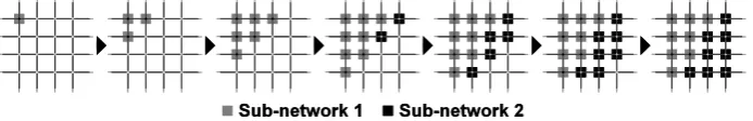
The MBFSMTL method considers the road traffic network as a weighted graph with crossroads acting as nodes and the sets of lanes inter-connecting the neighboring crossroads acting as edges. This graph is then explored from a staring crossroad using the breadth-first search algorithm. The crossroads are assigned to the particular sub-networks based on the actual sum of the weights of the explored edges (i.e. sets of traffic lanes). Once the entire traffic network is explored, the lanes connecting crossroads from different sub-networks are marked to be divided [15]. The exploration of the road traffic network is depicted in Fig. 1.
Fig. 1. The exploration of the road traffic network using MBFSMTL
Because the result of the division is significantly influenced by the selection of the starting crossroad, the entire process is performed from all crossroads of the traffic network. The division with the minimal number of divided traffic lanes is then selected [15].
4.3. GAMTL Method for Homogenous Clusters
The second method is the GAMTL (Genetic Algorithm Marking of Traffic Lanes). It employs a standard genetic algorithm for a multi-objective optimization [24] for the division of the road traffic network.
the higher its fitness value is. Once this value is calculated for entire population, a number of individuals are selected, crossed, and mutated in order to produce a new generation. This process repeats until a preset fitness value is reached or a preset number of generations is created [25].
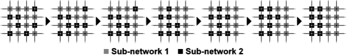
Using the GAMTL method, an individual is a specific assignment of the crossroads to the particular sub-networks. The fitness function represents the requirements on the solution – the load-balancing of the resulting sub-networks (called equability) and the minimal number of divided traffic lanes (called compactness). The ratio between these two parts of the fitness function can be set prior the road traffic network division similar to the number of generations and the number of mutations per individual [26]. The assignment of the crossroads to the particular sub-networks then changes using the crossover and mutation from a random pattern to clusters of crossroads (see Fig. 2).
Fig. 2. The change of the assignment of the crossroads using the GAMTL
The assignment of the crossroads to the particular sub-networks represented by the individual of the last generation with the highest fitness value is used for the division of the road traffic network. Similar to the MBFSMTL method, the lanes connecting the crossroads assigned to different sub-networks are marked as divided.
Based on the performed tests, the GAMTL method gives slightly better results. This means that the distributed simulation of the road traffic network divided by the GAMTL method is slightly faster (from 3 % to 22 %) than the simulation of the same traffic network divided by the MBFSMTL method [8]. On the other hand, the computation time of the MBFSMTL method is lower then the computation time of the GAMTL method. Hence, both methods seem to be utilizable [27].
5.
Division Methods for Heterogeneous Clusters
For the heterogeneous clusters, the methods originally developed for the homogenous clusters (see Section 4) must be modified.
5.1. Specifics of the Heterogeneous Cluster
Heterogeneous Clusters powers [28]. This makes the load-balancing of the road traffic sub-networks a little more complicated task. The division of the road traffic network into the sub-networks with similar number of vehicles (i.e. similar load) is impractical in this case [28]. Using such a division, the computational power of the slowest node would be fully utilized, but the faster nodes would have to wait for this slowest node to finish the computation in every time step.
Hence, it is necessary to take the computational power of each node of the heterogeneous cluster into the account during the road traffic network division. This means that each node is assigned by such a part of the road traffic network that the computation of one time step takes the similar time to all nodes. Then, the computational power of each node is fully utilized and the speed of the distributed simulation is maximized [27].
5.2. Necessary Modifications to the Division Methods
As mentioned in Section 5, the road traffic division methods developed for the homogenous clusters must be modified in order to be fully utilizable and efficient for the heterogeneous clusters.
Nevertheless, the assigning of the weights to traffic lanes used by both methods requires no modifications. In this computation, the data are only prepared for the marking of traffic lanes and no information about the target distributed computer it utilized. All three approaches to the weights assigning described in Section 3.1 could be used for the road traffic network division for the heterogeneous clusters. However, because all the approaches give similar results [21], [22], the fastest approach – the MaSBWA – will be used.
On the contrary, the modifications are necessary to the marking of traffic lanes of both methods. It is necessary to consider the various computational powers of the nodes of the heterogeneous cluster during the creation of the resulting sub-networks. This means that the load of the traffic network must not be divided uniformly among the resulting sub-networks, but rather in ratio, which corresponds to the ratio of the computational powers of the nodes of the cluster. However, this ratio is specific for each heterogeneous cluster and must be determined prior to the division of the road traffic network [27].
5.3. Investigation of the Speed of Heterogeneous Cluster Nodes
The first possible approach is the utilization of known parameters of the node, such as CPU frequency, size of the RAM, number of floating-point operations per second, and so on. Nevertheless, from this information, it is difficult to determine the resulting speed of the road traffic simulation performed on the node. This information is most important for the determination of the computational power ratio of the particular nodes. Some theoretical speed of the nodes is from this point of view irrelevant [27].
Hence, it is more convenient to use a set of tests (i.e. a benchmark) for determination of the speeds of the particular nodes of the heterogeneous cluster. These tests should utilize directly the road traffic simulation in order to obtain most relevant information about the speeds of the nodes. This approach is used for both our methods for the division of road traffic network for heterogeneous clusters [27].
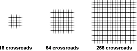
For the determination of the speed of each node of the heterogeneous cluster, the DUTS simulator (see Section 2.5) is used. Three road traffic networks were prepared to be performed on each node. The networks are regular grids of 16, 64, and 256 crossroads (see Fig. 3). The networks are small enough to keep the testing time in reasonable limits even on slower nodes and large enough to make the testing easily measurable [27].
Fig. 3. The road traffic networks used for benchmarking of each node
During the benchmark, ten simulation runs of each road traffic network are performed on every node of the heterogeneous cluster. The computation time and the mean number of vehicles moving within the road traffic network are observed during each simulation run. For each road traffic network and each node, the mean computation time and the mean number of vehicles are calculated. It has been determined that ten simulation runs for each combination of the node and road traffic network are sufficient. The mean deviation of each measured value from the mean value is under 1 % for the computation time and under 3 % for the mean number of vehicles moving within the traffic network [27].
Heterogeneous Clusters
3
31
j ijij
i
T
V
k
,(1)
where ki is the computational power coefficient of the ith node, Vij is the mean
number of vehicles of the jth road traffic network on the ith node, and Tij is
the mean computation time of the jth traffic network on the ith node. Using the coefficients, the portion of the load of each node can be calculated as:
Nj j i i
k
k
r
1
,
(2)
where ri is the portion of the load of the ith node, ki is the computational
power coefficient of the ith node, kj is the computational power coefficient of
the jth node, and N is the number of nodes. The calculated portions of the load of the particular nodes are then used for division of the load of the road traffic network among the sub-networks in ratio r1: r2 : … : rN.
5.4. MBFSMTL Method for Heterogeneous Clusters
Now, as we discussed the determination of the ratio, which will be used for division of the load among the road traffic sub-networks, we can proceed with the description of the methods for marking of traffic lanes for heterogeneous clusters. Both described methods for homogeneous clusters are viable for heterogeneous clusters as well, but with some modifications. The MBFSMTL method for heterogeneous clusters is described in this section. The GAMTL method for heterogeneous clusters is described in Section 5.5.
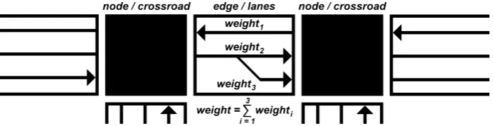
As it was said in Section 4.2, the MBFSMTL method utilizes a modified breadth-first search algorithm. The inputs of the method are the road traffic network with traffic lanes assigned with weights (see Section 4.1 and 5.2) and the portions of the load of the particular nodes (see Section 5.3). The road traffic network is considered as a weighted graph with crossroads acting as nodes of the graph and the sets of lanes connecting crossroads acting as weighted edges of the graph (see Fig. 4). Prior to the searching of the graph, the total weight of the divided traffic network is calculated as:
Li i
T
w
W
1
, (3)
where WT is the total weight of the divided traffic network, L is the number of
Fig. 4. Road traffic network as weighted graph (an input for division methods) Once the total weight of the road traffic network is determined, the aimed weights of particular sub-networks can be calculated. Unlike the MBFSMTL method for homogenous clusters, this number is not the same for all sub-networks, but must be calculated using the portions of the load of the particular nodes of the heterogeneous cluster as:
T i
Si
r
W
W
, (4)where WSi is the aimed weight of the ith sub-network, ri is the portion of the
load of the node, on which the simulation of the ith sub-network will be performed, and WT is the total weight of the divided traffic network. Also, the
current sub-network’s number is set to zero, the current sub-network’s current weight is set to zero, and the aimed weight of current sub-network is set to the first value of the aimed weights of the particular sub-networks (i.e. WS1).
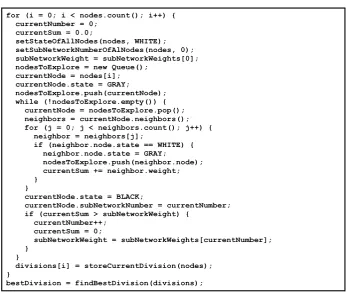
When all necessary values are initialized, a crossroad is selected as the starting node of the breadth-first search algorithm. The starting crossroad is assigned by the current sub-network’s number (zero at this point). As the breadth-first searching is performed, the explored crossroads are assigned with the current sub-network’s number and the weights of the explored edges are added to the current sub-network’s current weight. When this value reaches the aimed weight of the current network, the current sub-network’s number is incremented, the current sub-sub-network’s current weight is reset to zero, and the aimed weight of the current sub-network is set to the next value of the aimed weights of the particular sub-networks. These steps repeat until the entire road traffic network is explored [27].
When the entire road traffic network is explored, it means that all crossroads have been assigned with the number of road traffic sub-network. To mark traffic lanes, which shall be divided to create the sub-networks, it is sufficient to mark all traffic lanes connecting all pairs of the crossroads with different numbers of sub-networks [27].
Heterogeneous Clusters
Fig. 5. The algorithm of the MBFSMTL method for heterogeneous clusters
5.5. GAMTL Method for Heterogeneous Clusters
As it was said in Section 4.3, the GAMTL method utilizes a genetic algorithm. Similar to the MBFSMTL method, the GAMTL method utilizes the road traffic network with traffic lanes assigned with weights and the portions of the load of the particular nodes as its inputs.
Fig. 6. An individual with corresponding assignment of the crossroads
Once the initial population is generated, the fitness function is calculated for each individual. Similar to the homogenous GAMLT method, the fitness functions consists of two parts – the compactness and the equability.
The compactness is used for minimization of the number of divided lanes. It can be calculated as:
L
L
L
C
D, (5)
where C is the compactness, LD is total number of divided lanes, and L is the
total number of lanes. The compactness is calculated in the same way for both heterogeneous and homogenous clusters.
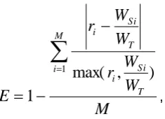
The only part of the GAMTL method, which is different for the heterogeneous clusters, is the calculation of the equability, which is used for correct distribution of the load among the sub-networks. For the heterogeneous clusters, the load of the road traffic network cannot be divided uniformly, but rather using the portions of the load of the particular nodes. Hence, the equability can be calculated as:
M
W
W
r
W
W
r
E
M
i
T Si i
T Si i
1
max(
,
)
1
,(6)
where E is the equability, WSi is the total weight of the ith sub-network using
the assignment of the crossroads corresponding to the individual, for which the equability is calculated, WT is the total weight of the road traffic network
(see Equation (3)), M is the number of sub-networks, and ri is the portion of
the load of the node, on which the simulation of the ith sub-network will be performed.
With both compactness and equability calculated, it is possible to calculate the entire fitness function as:
r
C
E
r
F
E
1
E
, (7)where F is the fitness function, C is the compactness, E is the equability and
Heterogeneous Clusters The rE determines the preference of the compactness (optimization of the
inter-process communication) or the equability (load-balancing of the sub-networks). For rE equal to 0, the GAMTL method is focused solely on the
compactness. So, the division with minimal number of divided lanes is found. However, the minimal possible number of divided lanes is zero, which happens in case that there is only one resulting sub-network (i.e. the traffic network is not divided at all). Since such a division is useless for our purposes, the rE should be greater than 0. For rE equal to 1, the GAMTL
method is focused solely on the load-balancing and the number of divided lanes is not taken into account. This setting is theoretically usable, because the required number of sub-networks is created. Nevertheless, a very high number of divided lanes is generated, because there is no component of the fitness function, which would prevent it. Hence, an intense inter-process communication and consequently a non-negligible reduction of the speed of the distributed simulation must be expected. Based on preliminary experiments with the settings of the rE, the default value is set to 0.25. With
this setting, the number of divided traffic lanes is sufficiently low for many instances and the resulting sub-networks are still well load-balanced.
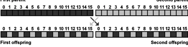
Once the fitness function is calculated for all 90 individuals, ten individuals with highest fitness function are selected for crossover using pairs of selected individuals. Each combination of two parent individuals produces two offspring (see Fig. 7). The first offspring receives integer values of even indices from the first parent and integer values of odd indices from the second parent. The second offspring receives all remaining values from both parents.
Fig. 7. The crossover of two parent individuals producing two offspring
The combination of all selected individuals produces a new generation of 90 individual. Each individual can be mutated. The mutation is limited to the maximum of five mutations per individual, which means that up to five values of each individual of the new generation can be randomly changed. Then, the fitness value is calculated for all individuals and the process repeats for 10 000 generations. All parameters of the GAMTL method for heterogeneous clusters (number of generations, number of individual, rE, etc.) were adopted
Once the genetic algorithm is completed, the traffic lanes connecting crossroads assigned to different sub-networks are marked as divided, similar to the MBFSMTL method.
6.
Tests and Results
Both described methods for heterogeneous clusters have been thoroughly tested. There were two sets of tests. The first set of tests (see Section 6.2) was the benchmark of the heterogeneous cluster, on which the distributed road traffic simulation was tested (see Section 5.3). This benchmark was performed prior the division of the road traffic networks, since its result (portions of the load) is a necessary input for both division methods for heterogeneous clusters. In the second set of tests (see Section 6.3), both division methods for heterogeneous clusters were tested and compared to their counterparts for homogenous clusters.
6.1. Heterogeneous Cluster Used for Testing
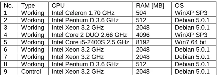
Both sets of tests were performed on a heterogeneous cluster consisting of nine nodes. Eight nodes were used as working nodes performing simulation of particular road traffic sub-networks. The remaining (control) node served as a centralized barrier for the synchronization of the working processes (see Section 2.4). The parameters are summarized in Table 1.
Table 1. Parameters of the nodes of the distributed cluster for testing
No. Type CPU RAM [MB] OS
1 Working Intel Celeron 1.70 GHz 504 WinXP SP3 2 Working Intel Pentium D 3.6 GHz 512 Debian 5.0.1 3 Working Intel Xeon 3.2 GHz 2048 Debian 5.0.1 4 Working Intel Core 2 DUO 2.66 GHz 4096 WinXP SP3 5 Working Intel Core i5-2400S 2.5 GHz 8192 Win7 64 bit 6 Working Intel Xeon 3.2 GHz 2048 Debian 5.0.1 7 Working Intel Xeon 3.2 GHz 2048 Debian 5.0.1 8 Working Intel Pentium D 3.6 GHz 512 Debian 5.0.1 9 Control Intel Xeon 3.2 GHz 2048 Debian 5.0.1
6.2. Benchmark of the Working Nodes of the Heterogeneous Cluster
sub-Heterogeneous Clusters networks, various numbers (two, four, and eight) of working nodes were used (see Section 6.3). Hence, the portions of the load were calculated for two working nodes (working nodes 1-2, control node 9), four working nodes (working nodes 1-4, control node 9), and eight working nodes (working nodes 1-8, control node 9).
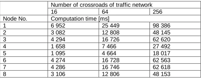
The benchmark was performed as follows. Sequential simulations of three road traffic networks (see Fig. 3) were performed ten times on each working node. Each simulation run was 900 time steps (corresponding to 15 minutes of the real time) long. Two values were observed in every simulation run – the mean number of vehicles moving within the road traffic network and the computation time of the simulation run. The computation times and the mean numbers of vehicles collected during ten simulation runs were then averaged and are summarized in Table 2 and Table 3, respectively.
As can be seen in Table 2, there are significant differences of the computation times of the same road traffic network simulated on different nodes. It can be observed that the computation time is not linearly dependent on the CPU frequency. Nevertheless, the results are consistent with the anticipated computational power of the particular nodes.
Table 2. The mean computation times of the simulation runs Number of crossroads of traffic network
16 64 256
Node No. Computation time [ms]
1 6 952 25 449 98 386
2 3 082 12 808 48 145
3 4 294 16 726 62 620
4 1 658 7 466 27 492
5 1 095 4 664 18 017
6 4 274 16 728 62 563
7 4 286 16 746 62 618
8 3 106 12 806 48 153
Lastly, it should be noted that the values for nodes 2 and 8 are very similar and the values for nodes 3, 6, and 7 are very similar as well. This is not a coincidence. The nodes 2 and 8 and the nodes 3, 6, and 7 are computers with identical parameters. So, it could be assumed that the results of the benchmark will be the same for all identical nodes. Nevertheless, in order to verify this assumption, the benchmark was performed on all nodes. This way, it was shown that the results for nodes 2 and 8 are nearly identical and the results for nodes 3, 6, and 7 are nearly identical as well (see Table 2). The maximal difference is less than 1 %.
one column are caused by the stochastic nature of the simulation. Due to this nature, even two simulation runs of the same road traffic network performed on the same node are slightly different.
Table 3. The mean number of vehicles of the simulation runs Number of crossroads of traffic network
16 64 256
Node No. Mean number of vehicles during simulation run
1 724 1 660 3 514
2 721 1 636 3 585
3 726 1 647 3 585
4 720 1 684 3 514
5 718 1 666 3 535
6 727 1 649 3 580
7 723 1 652 3 593
8 717 1 641 3 581
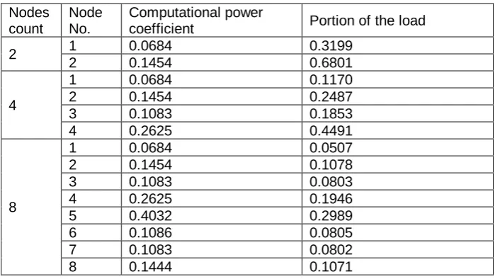
Based on the obtained values, the computational power coefficients and the portions of the load of each node for two, four, and eight utilized working nodes can be calculated using the Equation (1) and Equation (2), respectively. The results are summarized in Table 4. The portions of the load of the particular nodes were used as the input for both division methods for heterogeneous clusters.
Table 4. Computational power coefficients and portions of the load Nodes
count
Node No.
Computational power
coefficient Portion of the load
2 1 0.0684 0.3199
2 0.1454 0.6801
4
1 0.0684 0.1170
2 0.1454 0.2487
3 0.1083 0.1853
4 0.2625 0.4491
8
1 0.0684 0.0507
2 0.1454 0.1078
3 0.1083 0.0803
4 0.2625 0.1946
5 0.4032 0.2989
6 0.1086 0.0805
7 0.1083 0.0802
Heterogeneous Clusters
6.3. Performance of the Methods for Heterogeneous Clusters
The performances of the MBFSMTL and GAMTL methods for heterogeneous clusters were tested and compared to the performances of the MBFSMTL and GAMTL methods for homogenous clusters. Using this approach, it is shown that the consideration of the computational power of particular nodes of the heterogeneous cluster during the road traffic network division influences the resulting speed of the distributed road traffic simulation.
For the testing, four road traffic networks were used. Network 1 was an irregular road traffic network of 55 crossroads inspired by the Bory district of the Pilsen city, Czech Republic. Networks 2, 3, and 4 were regular square grids of 64, 256, and 1 024 crossroads, respectively. The networks were divided into two, four, and eight sub-networks using both methods for heterogeneous clusters and both methods for homogenous clusters. Then, the distributed microscopic road traffic simulation using the DUTS system was performed on two, four, and eight working nodes of the heterogeneous cluster (see Section 6.1), respectively.
For each combination of the divided road traffic network, the number of sub-networks, and the division method, ten simulation runs were performed and the computation time and the numbers of vehicles moving in particular sub-networks were observed. Similar to the benchmark, each simulation run was 900 time steps long, which corresponds to 15 minutes of the real time. This length of the simulation runs was selected, because the real data of the road traffic intensities in Pilsen city are collected in 15-minutes-long intervals. This enables an easier comparison of the results from the simulation with the real measured data in the future [27].
The averaged numbers of vehicles moving in particular sub-networks were used for investigation of the distribution of the total load among the particular sub-networks in the distributed road traffic simulation. The portions of the load of the particular sub-networks are compared to the intended values obtained from the benchmark (see Table 5 for the MBFSMTL and Table 6 for the GAMTL method).
As can be seen in Table 5 and Table 6, the real portions of the load of the particular sub-networks are similar (but not identical) to the intended values regardless the utilized division method. The mean differences between the intended and real portions are low for both methods – 8.5 % for the MBFSMTL method and 9.3 % for the GAMTL method. Hence, from this point of view, both methods give similar results. The reason for the observed differences between intended and real portions of the load is that the methods are not focused solely on load-balancing, but on the number of divided traffic lanes as well. Hence, both methods can produce a division, in which the load-balancing is not perfect, but the number of divided traffic lanes is low.
vary from 3 % to 50 %. Such a high variance can be observed, because the total computation time of the distributed simulation is not influenced solely by the load-balancing, but by the inter-process communication as well.
Table 5. Portions of load of particular sub-networks created by MBFSMTL method MBFSMTL method Number of crossroads
Nodes count
Node No.
Intended portion
55 64 256 1 024
Portions of the load
2 1 0.3199 0.2786 0.2521 0.2655 0.2513 2 0.6801 0.7134 0.7679 0.7345 0.7487
4
1 0.1170 0.1376 0.0989 0.0991 0.1084 2 0.2487 0.2218 0.2547 0.2669 0.2391 3 0.1853 0.1950 0.2001 0.1741 0.1719 4 0.4491 0.4456 0.4463 0.4599 0.4806
8
1 0.0507 0.0411 0.0551 0.0599 0.0479 2 0.1078 0.1112 0.1189 0.0996 0.0981 3 0.0803 0.0901 0.0761 0.0813 0.0816 4 0.1946 0.2139 0.2144 0.2034 0.2017 5 0.2989 0.2782 0.3007 0.3001 0.2916 6 0.0805 0.0751 0.0697 0.0911 0.0722 7 0.0802 0.0791 0.0718 0.0765 0.0709 8 0.1071 0.1113 0.0933 0.0881 0.1360
Table 6. Portions of load of particular sub-networks created by GAMTL method GAMTL method Number of crossroads
Nodes count
Node No.
Intended portion
55 64 256 1 024
Portions of the load
2 1 0.3199 0.3491 0.2992 0.2799 0.2751 2 0.6801 0.6509 0.7008 0.7201 0.7249
4
1 0.1170 0.1118 0.1203 0.1021 0.0977 2 0.2487 0.2193 0.2409 0.2764 0.2189 3 0.1853 0.1604 0.2130 0.1919 0.2044 4 0.4491 0.5085 0.4258 0.4296 0.4790
8
1 0.0507 0.0391 0.0611 0.0626 0.0433 2 0.1078 0.0961 0.1109 0.1089 0.1189 3 0.0803 0.0902 0.0727 0.0894 0.0788 4 0.1946 0.2005 0.2011 0.2107 0.2119 5 0.2989 0.2501 0.3107 0.2856 0.2999 6 0.0805 0.1055 0.0788 0.0765 0.0911 7 0.0802 0.0917 0.0809 0.0719 0.0688 8 0.1071 0.1268 0.0838 0.0944 0.0873
Heterogeneous Clusters road traffic network and the utilized division method. The numbers of divided traffic lanes are summarized in Table 8.
Table 7. Mean computation time of the simulation run Computation time [s] Nodes
count
Crossroads count
Homogenous Heterogeneous MBFSMTL GAMTL MBFSMTL GAMTL
2
55 29.7 25.5 22.9 21.1
64 32.9 24.8 23.0 21.8
256 66.3 66.5 58.3 54.2
1 024 207.0 216.8 193.2 197.9
4
55 15.7 12.4 9.7 8.9
64 19.0 12.1 11.5 9.5
256 25.1 27.9 21.2 19.7
1 024 76.9 96.6 72.6 74.0
8
55 8.9 8.1 6.3 6.0
64 10.1 8.4 6.4 5.2
256 16.2 16.9 13.2 12.5
1 024 49.5 56.9 42.1 47.7
Table 8. Numbers of divided traffic lanes
Number of divided traffic lanes Nodes
count
Crossroads count
Homogenous Heterogeneous MBFSMTL GAMTL MBFSMTL GAMTL
2
55 27 21 14 16
64 44 16 16 18
256 44 80 28 54
1 024 108 196 82 144
4
55 70 30 63 27
64 100 32 81 32
256 170 142 134 108
1 024 280 794 210 706
8
55 94 67 79 65
64 144 116 98 80
256 322 576 360 498
1 024 592 1 112 588 996
different sub-networks as their neighbors. This greatly increases the number of divided traffic lanes and affects the resulting computation time of the distributed simulation.
In order to investigate this behavior further, another set of tests was performed. Two largest traffic networks (network 3 – 256 crossroads and network 4 – 1 024 crossroads) were divided into four sub-networks using the heterogeneous GAMTL method with 10 000, 100 000, and 1 000 000 generations, respectively. The best achieved compactness, equability, and fitness value, the computation time necessary for the division, and the numbers of divided traffic lanes were observed during the division. The division was performed on the node 4 of the heterogeneous cluster (see Table 1 for parameters). Then, the distributed road traffic simulation of the four resulting sub-networks was performed ten times for each combination of the network and the number of generations on working nodes 1 to 4 and control node 9 (see Table 1 for parameters) and the mean computation time was determined. The results are summarized in Table 9.
As can be seen in Table 9, the best achieved compactness, equability, and fitness value increase with increasing number of generations. Consequently, the quality of division is improving with increasing number of generations. This means that the number of divided traffic lanes is lower (corresponds to compactness) and the resulting sub-networks are better load-balanced (corresponds to equability). Nevertheless, this improvement is minimal (see last two rows of Table 9) and for the price of significant increase of computation time necessary for road traffic network division (see sixth row of Table 9).
Table 9. Dependency of the heterogeneous GAMTL method on the generations count
Crossroads 256 1 024
Generations 104 105 106 104 105 106 Compactness 0.9007 0.9136 0.9265 0.8329 0.8381 0.8542 Equability 0.5777 0.7289 0.7445 0.7575 0.7615 0.7973 Fitness 0.8200 0.8674 0.8810 0.8150 0.8179 0.8310 Division time
[s] 46.2 422.1 4 159.1 180.8 1 699.0 15 795.0 Divided lanes 108 94 80 706 684 616 Simulation time
[s] 19.7 19.6 19.3 74.0 73.8 73.4
Heterogeneous Clusters were set using preliminary testing of the homogenous GAMTL method and were adopted by the heterogeneous version. The preliminary testing suggested that the setting was convenient. Nevertheless, for optimal settings, a more thorough testing of all combinations of the particular parameters would be required. Moreover, there are other features of the genetic algorithm, which can be also very important (e.g. type of crossover, type of selection, etc.). These features have not been investigated yet.
The optimal settings of all mentioned parameters and features of the genetic algorithm of the GAMTL method is outside the scope of this paper. Nevertheless, it is one of the main aims of our future work. More information can be found in [30].
7.
Conclusions
In this paper, we have described two methods for division of road traffic networks for heterogeneous clusters – the MBFSMTL and the GAMTL. Both these methods are based on their counterparts originally designed for homogenous clusters. The methods for heterogeneous clusters divide the load among the particular road traffic sub-networks using a ratio based on the computational powers of the particular nodes of the heterogeneous cluster. In order to calculate the ratio, all nodes of the target heterogeneous cluster are investigated for their computational powers using a benchmark test.
The performances of both methods for heterogeneous clusters were thoroughly tested and compared mutually and with their counterparts for homogenous clusters. Both methods for heterogeneous clusters showed better results then both methods for homogenous clusters for all tested instances. The savings of the computational time of the distributed simulation reached up to 50 %. Hence, it is clear that the adaptation of the load of particular sub-networks for the computational power of the nodes has a significant effect on the resulting computation time of the distributed simulation.
When both methods for heterogeneous clusters are compared together, the GAMTL method gives better results for smaller road traffic networks than the MBFSMTL methods. On the contrary, the MBFSMTL method gives better results for larger traffic networks, and shows more stable results due to the lower number of divided traffic lanes. At first glance, this makes the MBFSMTL method more utilizable than the GAMTL method. However, the worse results of the GAMTL method could be caused by suboptimal settings of the parameters of the utilized genetic algorithm. So, it is possible that, after an optimization, the GAMTL method will give better results than the MBFSMTL method.
Another step in our research is the combination of the described methods for the load-balanced division of road traffic networks with efficient communication protocols. For the testing of the division methods described in this paper, a basic (i.e. not optimized) communication protocol was used. However, we have developed several advanced communication protocols, which can significantly reduce the amount of inter-process communication [3]. Since the inter-process communication is relatively slow, the utilization of an advanced communication protocol can significantly improve the overall performance of the distributed road traffic simulation. Moreover, some of the advanced protocols could mitigate the higher number of divided traffic lanes produced by the division methods in some instances [3].
Another promising direction of our research is the parallel/distributed road traffic simulation, which can better exploit the computational powers of the nodes with multiple or multi-core processors than a pure distributed simulation due to the utilization of shared memory instead of message passing were possible [12].
References
1. Fujimoto, R. M.: Parallel and Distributed Simulation Systems. John Wiley & Sons, New York, USA. (2000)
2. Lighill, M. H., Whitman, G. B.: On kinematic waves II: A theory of traffic flow on long crowed roads. In Proceedings of the Royal Society of London, s. A, 229, London, United Kingdom. (1955)
3. Potuzak, T.: Methods for Reduction of Interprocess Communication in Distributed Simulation of Road Traffic. Doctoral thesis, University of West Bohemia, Pilsen, Czech Republic. (2009)
4. Nagel, K., Schreckenberg, M.: A Cellular Automaton Model for Freeway Traffic. In Journal de Physique I, 2, 2221–2229. (1992)
5. Gipps, P. G.: A behavioural car following model for computer simulation. In Transp. Res. Board, 15-B(2), 403–414. (1981)
6. Nagel, K., Rickert, M.: Parallel Implementation of the TRANSIMS Micro-Simulation. In Parallel Computing, Vol. 27, No. 12, 1611–1639. (2001)
7. Gonnet, P. G.: A Queue-Based Distributed Traffic Micro-simulation. Technical report. (2001)
8. Potuzak, T.: Methods for Division of Road Traffic Networks Focused on Load-Balancing. In Advances in Computing, Vol. 2, No. 4, 42–53. (2012)
9. Nizzard, L.: Combining Microscopic and Mesoscopic Traffic Simulators. Raport de stage d’option scientifique, Ecole Polytechnique, Paris, France. (2002) 10. Nagatani, T.: Gas Kinetic Approach to Two-Dimensional Traffic Flow. In J. Phys
Soc Jap, Vol. 65, No. 10, 3150–3152. (1996)
11. Burghout, W.: Hybrid microscopic-mesoscopic traffic simulation. Doctoral thesis, Royal Institute of Technology, Stockholm, Sweden. (2004)
Heterogeneous Clusters 13. Klein, U., Schulze, T., Strassburger, S., Menzler, H.: Distributed Traffic Simulation Based on the High Level Architecture. In Proceedings of Simulation Interoperability Workshop, Orlando, USA. (1998)
14. Kiesling, T., Lüthi, J.: Towards Time-Parallel Road Traffic Simulation. In Proceedings of the Workshop on Principles of Advanced and Distributed Simulation. (2005)
15. Potuzak, T.: Division of Traffic Network for Distributed Microscopic Traffic Simulation Based on Macroscopic Simulation. In Proceedings of the 7th EUROSIM Congress on Modelling and Simulation, Vol. 2, Prague, Czech Republic. (2010)
16. Barcelo, J., Ferrer, J. F., Garci, D., Florian, M., Le Saux, E.: The Parallelization of AIMSUN2 Microscopic Simulator for ITS Applications. In Proceedings of 3rd World Congress on Intelligent Transportation Systems, Orlando, Florida. (1996) 17. Hartman, D.: Leading Head Algorithm for Urban Traffic Model. In Proceedings of
the 16th International European Simulation Symposium ESS, Budapest, Hungary, 297–302. (2004)
18. Cetin, N., Burri, A., Nagel, K.: A Large-Scale Agent-Based Traffic Microsimulation Based on Queue Model. In Proceedings of 3rd Swiss Transport Research Conference, Monte Veritas. (2003)
19. Klefstad, K., Zhang, Y., Lai, M., Jayakrishnan, R., Lavanya, R.: A Scalable, Synchronized, and Distributed Framework for Large-Scale Microscopic Traffic Simulation. In The 8th International IEEE Conference on Intelligent Transportation Systems. (2005)
20. Wei, D., Chen, W., Sun, X.: An Improved Road Network Partition Algorithm for Parallel Microscopic Traffic Simulation. In 2010 International Conference on Mechanic Automation and Control Engineering, 2777–2782, Wuhan, China. (2010)
21. Potuzak, T.: Usability of Macroscopic and Mesoscopic Road Traffic Simulations in Division of Traffic Network for Distributed Micro-scopic Simulation. In CSSim 2011 – Conference on Computer Modelling and Simulation, Brno, Czech Republic, 94–101. (2011)
22. Potuzak, T.: Comparison of Road Traffic Network Division Based on Microscopic and Macroscopic Simulation. In UKSim 2011 – UKSim 13th International conference on Computer Modelling and Simulation, Cambridge, United Kingdom, 409–414. (2011)
23. Knuth, D. E.: The Art of Computer Programming Vol. 1. 3rd edition, Addison-Wesley. (1997)
24. Farshbaf, M., Feizi-Darakhshi, M.: Multi-objective Optimization of Graph Partitioning using Genetic Algorithms. In 2009 Third International Conference on Advanced Engineering Computing and Applications in Sciences, Sliema. (2009) 25. Menouar, B.: Genetic Algorithm Encoding Representations for Graph Partitioning
Problems. In 2010 International Conference on Machine and Web Intelligence (ICMWI), Algiers, 288–291. (2010)
26. Potuzak, T.: Utilization of a Genetic Algorithm in Division of Road Traffic Network for Distributed Simulation. In ECBS-EERC 2011 – 2011 Second Eastern European Regional Conference on the Engineering of Computer Based Systems, Bratislava, Slovakia, 151–152. (2011)
28. Bohna, C. A., Lamontb, G. B.: Load Balancing for Heterogeneous Clusters of PCs. In Future Generation Computer Systems, Vol. 18, No. 3, 389–400. (2002) 29. Potuzak, T.: Suitability of a Genetic Algorithm for Road Traffic Network Division.
In KDIR 2011 – Proceedings of the International Conference on Knowledge Discovery and Information Retrieval, Paris, France, 448–451. (2011)
30. Potuzak, T.: Issues of Optimization of a Genetic Algorithm for Traffic Network Division using a Genetic Algorithm. In KDIR 2012 – Proceedings of the International Conference on Knowledge Discovery and Information Retrieval, Barcelona, Spain, 340–343. (2012)
Tomas Potuzak was born in 1983 in Sušice, Czech Republic. He went to University of West Bohemia (UWB) where he studied software engineering and obtained his degree in 2006. Then, he entered Ph.D. studies at the Department of Computer Science and Engineering (DCSE) at the same university and has worked on issues of distributed simulation of road traffic. He obtained his Ph.D. in 2009. He is now a senior lecturer at the DCSE UWB. His research is focused on the issues of distributed simulations and component-based simulations.