Probabilistic Methods In Information Theory

CSUSB ScholarWorks

CSUSB ScholarWorks

Electronic Theses, Projects, and Dissertations Office of Graduate Studies

9-2016

Probabilistic Methods In Information Theory

Probabilistic Methods In Information Theory

Erik W. Pachas

Cal State University-San Bernardino

Follow this and additional works at: https://scholarworks.lib.csusb.edu/etd

Part of the Other Statistics and Probability Commons

Recommended Citation Recommended Citation

Pachas, Erik W., "Probabilistic Methods In Information Theory" (2016). Electronic Theses, Projects, and Dissertations. 407.

https://scholarworks.lib.csusb.edu/etd/407

A Thesis

Presented to the

Faculty of

California State University,

San Bernardino

In Partial Fulfillment

of the Requirements for the Degree

Master of Arts

in

Mathematics

by

Erik W. Pachas

A Thesis

Presented to the

Faculty of

California State University,

San Bernardino

by

Erik W. Pachas

September 2016

Approved by:

Dr. Yˆuichirˆo Kakihara, Committee Chair Date

Dr. Hajrudin Fejzic, Committee Member

Dr. Shawn McMurran, Committee Member

Dr. Charles Stanton, Chair, Dr. Corey Dunn Department of Mathematics Graduate Coordinator,

Abstract

Given a probability space, we will analyze the uncertainty, that is, the amount of

informa-tion of a finite system, by studying the entropy of the system. We also extend the concept

of entropy to a dynamical system by introducing a measure preserving transformation on

a probability space. After showing some theorems and applications of entropy theory, we

study the concept of ergodicity, which helps us to further analyze the information of the

Acknowledgements

First of all, I would like to express my great gratitude to my advisor Dr. Yˆuichirˆo

Kakihara. His patience, dedication and understanding have contributed greatly in order

to achieve my goal. I would like to thank the members of my committee, Dr. Hajrudin

Fejzic and Dr. Shawn McMurran, for taking the time to read and make any comments

or suggestions to improve this paper.

I would also like to thank the stuff from the math department for their support

and positive attitude, which has made this graduate school experience a pleasant

jour-ney. Especially, I would like to express my appreciation to Dr. Corey Dunn. His words

of encouragement and enthusiastic personality has influenced me to do my best during

all these years.

Finally, I would like to thank my family for their great support and contribution

to reach my goals. All this work and effort has been inspired and dedicated to my mother,

Table of Contents

Abstract iii

Acknowledgements iv

1 Shannon Entropy 1

1.1 Introduction . . . 1

1.2 Properties and Axioms . . . 1

1.3 Deriving The Entropy Function . . . 8

1.4 Additional Properties of Entropy and Coding Theory . . . 12

2 The Kolmogorov-Sinai Entropy 16 2.1 Introduction . . . 16

2.2 The Kolmogorov-Sinai Theorem . . . 16

2.3 Bernoulli and Markov Shifts . . . 22

3 Relative Entropy and Kullback-Leibler Information 26 3.1 Introduction . . . 26

3.2 Discrete Relative Entropy and Its Properties . . . 26

3.3 Continuous Entropy and Relative Entropy . . . 32

3.4 Birkhoff Pointwise Ergodic Theorem . . . 37

4 Conclusion 41

Chapter 1

Shannon Entropy

1.1

Introduction

The concept of entropy is used in different fields of study such as

thermody-namics, statistical mechanics, and communication theory, just to name a few. In

ther-modynamics, entropy is an indicator of reversibility. That is, when there is no change of

entropy, the process is reversible. The unpredictability based on a lack of knowledge of

positions and velocities of molecules is given by the entropy in statistical mechanics. Now,

a different perspective of entropy is given in communication theory. Here we consider a

message source, such as a writer or speaker. The amount of information conveyed by

the message increases as the amount of uncertainty as to what message actually will be

produced becomes greater [Pie80]. Thus, in general, we can state that entropy measures

the amount of information given by a source, and a way to describe that source is using

ergodicity. These two concepts are part of a bigger spectrum called information theory

and this theory will be developed using concepts of probability theory, which will help us

to generalize and understand it mathematically.

1.2

Properties and Axioms

Definition 1.2.1. Let n∈_N and X ={x1, ..., xn} be a finite set with probability

distri-bution p = (p1, ..., pn). That is, 0 ≤pj = p(xj) ≤ 1, and these probabilities also satisfy

the condition that

n

P

j=1

pj = 1. We usually denote this as (X, p) and call it a complete

The entropy or the Shannon entropy H(X) of a finite scheme(X, p) is defined by

H(X) =−

n

X

j=1

pjlogpj.

We say that H(X) is the measure of uncertainty or information of the system (X, p).

We will use the convention that 0 log 0 = 0, which is easily justified by continuity

since xlogx →0 as x →0. Also, notice that adding terms of zero probability does not

change the entropy. If the base of the logarithm is b, we denote the entropy asHb(X).

A common units of entropy measure are base 2 and e. If the base of the logarithm is e,

the entropy is measured in nats. And, if the base of the logarithm is 2, the entropy is

measured in bits. Furthermore, note that entropy is a functional of the distribution ofX. Consequently, it does not depend on the actual values taken by the random variable X, but only on the probabilities [CT06].

Example 1.2.1. Bernoulli EntropyLet X={0,1} be a random variable with a prob-ability distribution p(x1 = 0) = 1−p and p(x2 = 1) = p. Then its entropy is given

by

H2(X) =−plogp−(1−p) log(1−p).

If we differentiate the entropy function H2(X) with respect to p, we find that H20(X) =

H₂0(p) = −_log1

e2(logep−loge(1−p)) = 0 when p = 1/2. That is, the entropy H2(X)

attains its maximum value of 1 bit at p= 1/2.

Example 1.2.2. Geometric EntropyAssume that we perform a number of independent trials until a success happens with probability p. We define the random variable X to be the number of trials required until the first success. Then X is known as a geometric random variable with parameter p and probability distribution

p(X=n) = (1−p)n−1p, n= 1,2, ...

Then we find the entropy of X,

H2(X) =− ∞

X

n=1

=− "

plog(1−p)

∞

X

n=1

(n−1)(1−p)n−1+plogp

∞

X

n=1

(1−p)n−1 #

=− "

p(1−p) log(1−p)

∞

X

n=0

n(1−p)n−1+plogp

∞

X

n=0

(1−p)n #

=− "

−plog(1−p)

∞

X

n=1

d

dp(1−p)

n_+plogp 1

1−(1−p) #

=− "

−plog(1−p) d dp

∞

X

n=1

(1−p)n+plogp p

#

=−p(1−p) log(1−p) 1 p2 −

plogp p

= −(1−p) log(1−p)−plogp

p .

Example 1.2.3. Poisson Entropy A random variable X = {0,1,2, ...} is said to be Poisson with parameter λ if for someλ >0,

p(xi =i) =e−λ

λi

i! i= 0,1, ...

If we calculate the entropy over all the possible values of a Poisson random variable, then we have

He(X) =−

∞

X

i=0

e−λλ

i

i! loge

−λλi

i!

=−e−λ "_∞

X

i=0

λi i!(loge

−λ_{+ logλ}i_−logi!)

#

=−e−λ "_∞

X

i=0

λi

i!(−λ) +

∞

X

i=0

λi

i!(ilogλ)−

∞

X

i=0

λi i! logi!

#

=−e−λ "

−λeλ+λ

∞

X

i=1

λi−1

(i−1)!(logλ)−

∞

X

i=0

λi i! logi!

#

=−e−λ "

−λeλ+λeλlogλ−

∞

X

i=0

λi i! logi!

#

=λ(1−logλ) +e−λ

∞

X

i=0

λi i! logi!.

Thus, the entropy of a random variable with Poisson distribution is given by He(X) =λ(1−logλ) +e−λ

∞

X

i=0

Because the entropy is calculated using the probabilities of each value of the

random variable, we can easily show thatH(X)≥0. We get this property since 0≤pi≤

1, which implies that −logpi ≥0. Given this fact, we can state that the minimum value

of H(X) is 0, and that this minimum value is achieved whenever we have pi = 0 or 1.

Can we also talk about a maximum value ofH(X) given this finite scheme? We will first

claim that H(X)≤lognassuming that X is taking overndistinct finite values. Before

we prove our claim, we will define the set of probability distribution, and then prove a

lemma in [Ash67].

Definition 1.2.2. For n ∈ _N, ∆n denotes the set of all probability distributions p =

(p1, ..., pn), i.e.,

∆n=

 



p= (p1, ..., pn) : n

X

j=1

pj = 1, pj ≥0,1≤j≤n

 

 .

Lemma 1.2.1. Let p, q∈∆n. Then n

X

j=1

pjlogqj ≤ n

X

j=1

pjlogpj,

where the equality is true when pi=qi, 1≤i≤n.

Proof. Because of the convexity of logx function, we know that logx≤x−1. Then using this inequality, we have

log qj pj

≤ qj pj

−1 or pjlog

qj

pj

≤pj

qj

pj

−pj for j= 1, ..., n.

Given that

n

P

j=1

pj = n

P

j=1

qj = 1, we obtain

n

X

j=1

pjlog

qj pj ≤ n X j=1

(qj−pj) = 0.

Thus _n

X

j=1

pjlog

qj pj = n X j=1

pjlogqj− n

X

j=1

pjlogpj ≤0.

And, the equality follows from the fact that logx=x−1 if and only ifx= 1.

Theorem 1.2.1. Let X={x1, ..., xn} be a random variable with probability distribution

p= (p1, ..., pn). Then

where the maximum value is attained if we have equally likely events, that is, pi = 1_n,

1≤i≤n.

Proof. Applying the previous lemma, we have H(X)−logn=−

n

X

j=1

pilogpi− n

X

j=1

pilogn

=−

n

X

j=1

pilogpi+ n

X

j=1

pilog

1 n

≤0,

which shows that H(X) ≤ logn. Note that if the random variable X has probabilities

pj = 1_n forj= 1, ..., n,

H(X) =H(1 n, ...,

1 n) =−

n

X

j=1

1 nlog

1

n = logn,

which is the maximum value for H(X).

Based on the theorem, we can answer with certainty that there is a maximum

value for H(X) = logngiven a finite scheme of noutcomes.

Since entropy measures that amount of uncertainty, it is important to define the

entropy involving two random variables. If we let Y ={y1, ..., ym} be another finite set,

then we define the following:

Definition 1.2.3. Let X and Y be two random variables. The pair (X, Y) with joint distribution p(x, y) has a joint entropy defined as

H(X, Y) =−X

x∈X

X

y∈Y

p(x, y) logp(x, y).

Definition 1.2.4. The conditional entropy H(X|Y) of X given Y is defined by

H(X|Y) =−X

y∈Y

X

x∈X

p(y)p(x|y) logp(x|y),

and we define conditional entropy of X given an observed value of Y =y, by

H(X|y) =−X

x∈X

Definition 1.2.5. For two random variables X and Y with a joint distribution p(x, y), the mutual information I(X, Y) between them is defined by

I(X, Y) =X

x,y

p(x, y) log p(x, y) p(x)p(y).

Notice if X and Y are independent random variables then the mutual infor-mation between them I(X, Y) = 0. Now, if we want to find the amount of mutual information between the random variable X and itself, we see that I(X, X) = H(X),

i.e., the self-mutual information is the entropy ofX. Using the above definition, we can easily prove the following:

I(X, Y) =H(X)−H(X|Y)

=H(Y)−H(Y|X)

=H(X) +H(Y)−H(X, Y).

As we mentioned before, the measure of dependence betweenXandY is relevant

to the computation of themutual information I(X, Y) as well as the entropy. As another example, suppose that we know that Y gives all the information about X. Then we

have that the measure of the entropy of X given Y is zero,H(X|Y) = 0, and it follows

that there is no change of uncertainty of X given Y. The next theorem will give some

important inequalities and illustrate the importance of dependence in order to arrive to

equality.

Theorem 1.2.2. Let p, q∈∆n be the probability distributions of X and Y respectively.

Then

i. H(X, Y)≤H(X) +H(Y)

ii. H(X|Y)≤H(X)

In both cases, equality holds true if and only if the random variables X and Y are inde-pendent.

H(X) +H(Y) =− X

x

p(x) logp(x) +X

y

p(y) logp(y) !

=− X

x

X

y

p(x, y) logp(x) +X

x

X

y

p(x, y) logp(y) !

=−X

x

X

y

p(x, y) logp(x)p(y)

≥ −X

x

X

y

p(x, y) logp(x, y), by lemma 1.4.1,

=H(X, Y).

The equality holds if and only ifp(x, y) =p(x)p(y) for allx, y if and only if X

and Y are independent.

(ii) First we claim that the compound entropy can be written as H(X, Y) =

H(Y)−H(X|Y). By definition we know that

H(X|Y) =−X

y∈Y

X

x∈X

p(y)p(x|y) logp(x|y)

=−X

y∈Y

X

x∈X

p(x, y) logp(x, y) p(y)

=−X

y∈Y

X

x∈X

p(x, y)(logp(x, y)−logp(y))

=− X

y∈Y,x∈X

p(x, y) logp(x, y) + X

y∈Y,x∈X

p(x, y) logp(y)

=H(X, Y)−H(Y).

This shows that the equation above is true. Now suppose that X andY are independent

random variables. Then

H(X|Y) =H(X, Y)−H(Y)

=H(X) +H(Y)−H(Y), by (i),

If the random variablesX andY are not independent, then

H(X|Y) =H(X, Y)−H(Y)

< H(X) +H(Y)−H(Y), also by (i),

=H(X).

Thus, we also proved the inequality in (ii).

1.3

Deriving The Entropy Function

After stating and proving several properties of the entropy functionH(X), we

want to show that the definition for such function makes sense and it is well-defined. In

order to do this, we list three more properties that uniquely define the entropy function

[Rom92].

i. H(p1, ..., pn) is defined and continuous for all p1, ..., pn, where 0 ≤ pi ≤ 1 for i=

1, ..., n and Pn

i=1pi = 1. We want this function to be continuous so that small

change in probabilities will result in a small change in uncertainty.

ii. H _n1, ...,1_n < H_n+11 , ...,_n+11 . This property tells us that the uncertainty in-creases as the number of outcomes inin-creases, outcomes that are equally likely to

occur. In fact, this entropy of equal likelihood is a monotonically increasing

func-tion.

iii. For ci∈Nand Pki ci=n, we have

H

1 n, ...,

1 n

=Hc1 n, ...,

ck

n

+

k

X

i=1

ci

nH

1 ci

, ..., 1 ci

.

To construct this equation, let the setX={x1, ..., xn}be partitioned into nonempty

disjoint subsets C1, ..., Ck. Let the size of each subset be |Ci|= ci for i= 1, ..., k,

and Pk

i=1ci =n. Now, let us choose a subset Ci with probability proportional to

subsetCi with equal probability. If the elementxj is in the subsetCu, then because

P(xj|Ci) =

  

 

0 ifi6=u 1

cu

ifi=u

we have

P(xj) = n

X

i=1

P(xj|Ci)P(Ci) =

1 cu cu n = 1 n.

This shows that if we choose xj this way, the probability will be the same as if we

were to choose directly from the whole setX with equal probability. Consequently,

the uncertainty of the outcomes remains the same.

If we choose directly from X with equal probability, the uncertainty will be

H

1 n, ...,

1 n

.

But now if we choose one of the subsetsC1, ..., Ck, the uncertainty is

H c₁

n, ..., ck

n

.

Now, once we have chosen the subset, we still have the uncertainty of choosing an

element from that subset. Then the average uncertainty in choosing an element is

k

X

i=1

P(Ci) ˙H

1 ci

, ..., 1 ci = k X i=1 ci nH 1 ci

, ..., 1 ci

.

Therefore, we have

H

1 n, ...,

1 n

=Hc1 n, ...,

ck n + k X i=1 ci nH 1 ci

, ..., 1 ci

.

Theorem 1.3.1. A functionH satisfies properties (i)-(iii) if and only if it is of the form

Hb(p1, ..., pn) =− n

X

i=1

pilogpi

Proof. Suppose that a functionHsatisfies all three properties mentioned above. Now, pick some positive integers m and n such that m divides n and ci = m for all

i= 1, ..., k. Because mk=Pk

i=1ci =n, we getk= _mn and using property (iii) gives

H

1 n, ...,

1 n

=Hm n, ...,

m n + k X i=1 m nH 1 m, ...,

1 m

=Hm n, ...,

m n +H 1 m, ...,

1 m k X i=1 m n

=Hm n, ...,

m n +H 1 m, ...,

1 m

.

Now, let n = ms where s is also a positive integer. Then the above equation

becomes

H

1 ms, ...,

1 ms =H 1 ms−1, ...,

1 ms−1

+H

1 m, ...,

1 m

.

Define the function f(n) =H _n1, ...,_n1. Now, we have

f(ms) =f(ms−1) +f(m)

=f(ms−2) +f(m) +f(m)

=f(m) +· · ·+f(m)

=sf(m).

And, this is true for all positive integersm and s. Because of property (ii), we

now get

f(ms)< f(ms+1),

sf(m)<(s+ 1)f(m).

It follows that f(m) must be a positive function. Let us choose some positive numbers

r, t and sso that

ms≤rt< ms+1

Then because f is a monotonically increasing function,

sf(m)≤tf(r)<(s+ 1)f(m)

s t ≤

f(r) f(m) <

s+ 1 t .

Also, we have

slogm≤tlogr <(s+ 1) logm,

s t ≤

logr logm <

s+ 1 t .

From the last two inequalities, we will get

−1 t ≤

f(r) f(m)−

logr logm <

1 t.

Now sincet was arbitrarily chosen, we must have

f(r) f(m) =

logr logm

or

f(r) logr =

f(m) logm

Since this is true for all positive integersr, we have

f(r) =Clogr for some C >0

since we also know that f(r) > 0. Now suppose that C = 1 by choosing the

base bof the logarithm appropriately. Then

f(r) = log_br for all r >0.

By property (iii),

H(c1 n, ...,

ck

n) =f(n)−

k

X

i=1

ci

nf(ci)

= log_bn−

k

X

i=1

ci

nlogbci

=

k

X

i=1

ci

nlogbn−

k

X

i=1

ci

n logbci

=−

k

X

i=1

ci

=−

k

X

i=1

ci

n logb ci

n.

Since any rationalp1, ..., pk ∈(0,1) can be expressed in the form c_n1, ...,c_nk , we

have

Hb(p1, ..., pk) =− k

X

i=1

pilogbpi.

But we also know that H is a continuous function so this must also hold for

all positive real numbers p1, ..., pk. Next, we will show that plogp = 0 if p = 0. For

simplicity, let log be the natural logarithmic function of base eand notice that

lim

p→0+plogp= lim_p→0+

logp 1/p

= lim

p→0+

1/p −1/p2

= 0.

Therefore,

Hb(p1, ..., pk) =− k

X

i=1

pilogbpi

holds for all nonnegative real numbers p1, ..., pk where 0 ≤ pi ≤ 1 and Pk_i=1pi = 1 for

i= 1, ..., k. For the converse, it is straight forward to show that the entropy functionH

satisfies the three properties mentioned above.

1.4

Additional Properties of Entropy and Coding Theory

To finish this section, we will present an inequality involving binomial

coeffi-cients, which plays an important role not only in information but also in coding theory.

In fact, this inequality is very useful in order to proveThe Noisy Coding Theorem[Rom92].

Lemma 1.4.1. Define the entropy function

Hq(λ) =λlogq

1

λ+µlogq 1 µ

for 0≤λ≤1 and µ= 1−λ. Then for any integer q≥2, we have

Proof. Ifq ≥2, then

qHq(λ)_=qλlogqλ1+µlogq µ1

=qλlogqλ1qµlogq

1

µ

= 2λlog2 1λ2µlog2

1

µ

= 2λlog2 1λ+µlog2µ1

= 2H(λ).

Theorem 1.4.1. Let H(λ) =λlog1_λ + (1−λ) log₍₁₋1_λ), where 0≤λ≤ 1₂. Then

bλnc

X

k=0

n k

≤2nH(λ)

where n_k is the binomial coefficient and the upper limitbλncof the summation is largest integer smaller or equal to nλ if nλ is not an integer.

Proof. We first observe that inequality holds trivially on the endpoints of the values ofλ. Specifically, ifλ= 0, thenH(0) = 0 and both sides of the inequality equal to

1. Now, if λ= 1/2, we have thatH(1/2) = 1 and that inequality becomes 2≤2n, which

is true forn≥1. Now, suppose that 0< λ <1/2.

From the Markov’s Inequality, we know if X is a random variable that takes only

non-negative values, then for any value a >0

P(X≥a)≤ E(X) a .

Let us assume that X has the form X = etY, where Y is a random variable, and t is a

real number. If we set a=etb, then it becomes

P(etY ≥etb)≤ E(e

tY₎

etb for all b∈R.

Now, ift <0, then we haveetY < etb if and only iftY ≥tbif and only if Y ≤b,

and so this is equivalent to

P(Y ≤b)≤ E(e

tY₎

IfY is a binomial random variable, with parameters (n, p), then

P(Y ≤b) =

b

X

k=0

n k

pkqn−k

whereq= 1−p. Furthermore,E(etY) is the binomial moment generating function, which

is well known to be

E(etY) = (q+pet)n.

Thus,

b

X

k=0

n k

pkqn−k≤e−tb(q+pet)n.

Settingb=λn, where 0< λ <1, we get

b

X

k=0

n k

pkqn−k ≤e−λnt(q+pet)n (1.1)

valid for t < 0. Let x= et and f(x) =x−λn(q+px)n. Since t < 0, we will minimizef over 0< x <1. By differentiatingf with respect tox, we get

f0(x) =nx−λn−1(q+px)(n−1)[−λ(q+px) +px].

Thus, the value ofx that will minimizef is

x= λq µp

where µ= 1−λ, and λ < p. Substituting this value ofx intof gives

λq µp

−λn

q+pλq µp

n =

λq µp

−λn qn

1 +λ

µ n

=

λq µp

−λn q µ

n

=λ−λnµ−µnpλnqµn

and (1.1) becomes

λn

X

k=0

n k

forλ < p. Settingp=q = 1₂ gives

λn

X

k=0

n k

≤λ−λnµ−µn

for λ < 1₂. From 1.4.1, we know λ−λnµ−µn = 2n[−λlogλ−µlogµ] = 2nH(λ), and the above inequality becomes

λn

X

k=0

n k

Chapter 2

The Kolmogorov-Sinai Entropy

2.1

Introduction

In the previous chapter, we developed Shannon’s way of measuring the infor-mation of a system. This notion of measuring the amount of uncertainty of source,

represented as a random variable along with its distribution, provided us with a

proba-bilistic way of quantifying the amount of uncertainty, and we called this entropy. Now,

in this chapter, we extend the concept of the entropy to a dynamical system, which is a

description of a physical system and its evolution over time. Therefore, we introduce the

concept of measure preserving dynamical systems and measure its unpredictability. We

will be able to state how unpredictable is a dynamical system depending on its entropy.

The higher the unpredictability, the higher the entropy. Furthermore, we will be able to

determine how the structure of two dynamical systems relates, i.e., whether or not two

dynamical system are isomorphic. To start, we will define some basic concepts and a

probability measure, found in [Shr04], so that we can define a dynamical system.

2.2

The Kolmogorov-Sinai Theorem

Definition 2.2.1. LetX be an arbitrary set. A collectionXof subsets ofXis aσ-algebra of X if

i. X ∈X;

iii. If(An:n∈N)⊂X, then Sn∈NAn∈X.

Definition 2.2.2. Let X be an arbitrary set, and X be a σ-algebra of X. A function

µ:X7→[0,1] is a probability measure if it satisfies the following properties: i. µ(∅) = 0;

ii. µ(X) = 1;

iii. For every disjoint sequence (An:n∈N) in X, we have µ

∞

[

i=1

Ai

! =

∞

X

i=1

µ(Ai).

Definition 2.2.3. Let (X,X, µ) be a probability measure space, and S :X → X. The transformation S is said to be measurable if S−1X ⊆ X. That is, S−1A ∈ X for every

A∈X. LetS be measurable. Then S is called a measure preserving transformation with respect to µ if

µ(S−1(A)) =µ(A) for every A∈X.

Definition 2.2.4. Let (X,X, µ) be a probability measure space, and let S : X → X

be a one-to-one measure preserving transformation. If S−1 is measurable, that is, S is invertible, then

S−1X=X=SX

andS−1 is also a measure preserving transformation. Now, the space(X,X, µ, S)is called a dynamical system, where S is measure preserving and not necessarily invertible.

Definition 2.2.5. Let 1 ≤ p < ∞. We say that the space Lp(X,X, µ) consists of all complex-valued measurable functions f on X that satisfy

Z

X

|f(x)|p_dµ(x)<∞.

Then, iff ∈Lp(X,X, µ), we define the Lp norm of f by

kfkp=

Z

X

|f(x)|pdµ(x) 1/p

If we let p= 1, the space L1_{(X,X, µ) consists of all integrable functions on X,}

Definition 2.2.6. For our purpose, we denote L1-space of (X,X, µ) by L1(X). IfY is a

σ-subalgebra of X andf ∈L1(X), let

µf =

Z

A

f dµ, A∈Y.

We notice that µf is a countably additive measure on Yand is absolutely

con-tinuous with respect to µ. That is, if A ∈ X and µ(A) = 0, then µf(A) = 0. By

Radon-Nikod´ym Theorem, there is a unique Y-measurable function g∈L1(Y) such that

µf =

Z

A

g dµ, A∈Y.

g is unique in theµ-a.e. sense. If we denote g=E(f|Y), theng is called the conditional

expectation of f relative toY. If we letf = 1A be the indicator function ofA∈X, then

we denote E(1A|Y) = P(A|Y), which is the conditional probability of A relative to Y

[Kak99].

Definition 2.2.7. Let Y be a σ-subalgebra ofX. AY-partition is a finiteY-measurable partition Aof X. That is,

1. A={A1, ..., An} ⊆Y,

2. Aj∩Ak=∅ if j6=k,

3. Sn

j=1Aj =X.

Definition 2.2.8. Consider the dynamical system (X,X, µ, S) and let the set of all

Y-partitions be denoted by P(Y). If we let A,B ∈ P(Y), then we define the following

Y-partitions:

A∨B={A∩B:A∈A, B∈B}

and

S−1A={S−1A:A∈A}

Now, let us define the partition

n−1

_

j=0

Definition 2.2.9. Let A ={A1, ..., An} ∈ P(X). The entropy H(A) of a partition A is

defined by

H(A) =−

n

X

j=1

µ(Ai) logµ(Ai)

=−X

A∈A

µ(A) logµ(A).

If we let the entropy function I(A) of A be defined by

I(A)(·) =−X

A∈A

1A(·) logµ(A),

then we have

H(A) =E(I(A)) = Z

X

I(A)dµ.

Definition 2.2.10. We define the conditional entropy function I(A|Y) as

I(A|Y)(·) =−X

A∈A

1A(·) logP(A|Y)(·).

Also, the conditional entropy H(A|Y) is defined by

H(A|Y) =E(I(A|Y)) = Z

X

I(A|Y)dµ. (2.1)

Since the entropy H(A) of a finite partitionA∈ P(X) can be expressed as the

Shannon Entropy, we also express the conditional entropyH(A|Y) as H(A|Y) =E(I(A|Y))

=E(E(I(A|Y)|Y))

=−X

A∈A

Z

X

P(A|Y) logP(A|Y)dµ.

Definition 2.2.11. Let A∈ P(X). Denote A˜ =σ(A), which is the σ-algebra generated by A. That is, A˜ is the smallest σ-subalgebra of X that contains A. Also, if Y₁,Y₂ are

σ-subalgebras, then let us denote Y₁∨Y₂=σ(Y₁∪Y₂), i.e., theσ-algebra generated by the union of Y₁ and Y₂.

Notice that P(A|B˜) = P

B∈B

µ(A|B)1B for A ∈ X, where µ(A|B) is the

condi-tional probability of A given B. Then we define

H(A|B˜) = X

B∈B

µ(B)X

A∈A

where − P

A∈A

µ(A|B) logµ(A|B) is the conditional entropy of A given B ∈ B and the

above equation is the average conditional entropy of Agiven B.

We also say that A≤B means thatB is finer than A, that is, each A∈A can

be expressed as a union of some elements in B.

Next, we state some fundamental theorems and lemmas so that we can prove

the Kolmorogov-Sinai Entropy theorem.

Theorem 2.2.1. Let A,B∈P(X) andY, Y1, Y2 be σ-subalgebras of X.

1. H(A|{∅, X}) =H(A).

2. H(A∨B|Y) =H(A|Y) +H(B|A˜ ∨Y). 3. H(A∨B) =H(A) +H(B|A˜).

4. A≤B⇒H(A|Y)≤H(B|Y). 5. A≤B⇒H(A)≤H(B).

6. Y2⊆Y1⇒H(A|Y1)≤H(A|Y2).

7. H(A|Y)≤H(A).

8. H(A∨B|Y)≤H(A|Y) +H(B|Y). 9. H(A∨B)≤H(A) +H(B).

10. H(S−1A|S−1Y) =H(A|Y). 11. H(S−1A) =H(A).

12. I(S−1A|S−1Y) =I(A|Y)◦S. 13. I(S−1A) =I(A)◦S.

Definition 2.2.12. Let A∈P(X). The entropy H(A, S) of S relative to Ais defined by

H(A, S) = lim

n→∞

1 nH





n−1

_

j=0

S−jA



We also define H(S) of S or the Kolmogorov-Sinai entropy ofS by

H(S) = sup{H(A, S) :A∈P(X)}.

Theorem 2.2.2. Let A,B∈P(Y). Then

H(A, S)≤H(B, S) +H(A|B˜).

Lemma 2.2.1. If Yn ↑Yand A∈P(X), then:

1. I(A|Y_n)→I(A|Y) µ-a.e. and in L1. 2. H(A|Yn)↓H(A|Y).

Theorem 2.2.3. (Kolmogorov-Sinai). If S is invertible and A ∈ P(X) is such that

∞

∨

n=−∞S

n_{A˜ =X, then H(S) =H(A, S).}

Proof. LetA_n= ∨n

k=−nS

k_{A forn≥1. Then}

H(An, S) = lim p→∞

1 pH

p−1

∨

j=0S −j_A

n

= lim

p→∞

1 pH

p−1

∨

j=0S −j

n

∨

k=−nS k_A

= lim

p→∞

1 pH

Sn

_p+2n−1 ∨

j=0 S −j_A

= lim

p→∞

p+ 2n−1 p

1 p+ 2n−1H

p+2n−1

∨

j=0 S −j_A

=H(A, S).

Now, letB∈P(X). Then,

H(B, S)≤H(An, S) +H(B|A˜n), theorem 2.2.2,

=H(A, S) +H(B|A˜n)

→H(A, S) (n→ ∞),

sinceH(B|A˜_n)↓H(B|X) by lemma 2.2.1 (2) and notice thatH(B|X) = 0. This

means that H(B, S)≤H(A, S) for B∈P(X), which implies that

TheKolmogorov-Sinai theorem provides us with a way to calculate the entropy H(S) of an invertible transformationS by calculating the entropyH(A, S) of that

invert-ible transformation S relative to a particular partition A of X. Moreover, this theorem

will help us to compute the entropy of Bernoulli shifts and Markov shifts [Kak99].

2.3

Bernoulli and Markov Shifts

We also want to study various dynamical systems and their entropies. Thus, we

would like to know if these systems are isomorphic or not.

Definition 2.3.1. Let (Xi,Xi, µi, Si) (i= 1,2)be two dynamical systems. These systems

are said to be isomorphic, denoted S1 ∼= S2, if there exists some one-to-one and onto

mapping ϕ:X1 →X2 such that

i. for any subset A1⊆X1, A1 ∈X1 iff ϕ(A1)∈X2, andµ1(A1) =µ2(ϕ(A1));

ii. ϕ◦S1=S2◦ϕ, that is, ϕ(S1x1) =S2ϕ(x1) for x1∈X1.

In this case, ϕ is called an isomorphism.

As a matter of fact, ifS1∼=S2, thenH(S1) =H(S2). That is, the

Kolmogorov-Sinai entropy of measure preserving transformations is invariant under isomorphism. Consequently, if H(S1) 6= H(S2), then S1 S2. Next, we define and compute the

entropy of Bernoulli and Markov shifts.

Example 2.3.1. Bernoulli Shifts. Let(X0, p)be a finite scheme, whereX0={a1, ..., al}

and p = (p1, ..., pl) ∈∆l, so that p(aj) = pj, 1 ≤j ≤ l. Consider the infinite Cartesian

product

X=XZ

0 ={x= (..., x 0

−1, x00, x 0

1, ...) :xk∈X0, k∈Z},

where Z={0,±1,±2, ...}, and the shift S on X given by S: (..., x−1, x0, x1, ...)7→(..., x0−1, x00, x

0

1, ...),where x 0

A cylinder set is defined by

[x0_i · · ·x0_j] ={(..., x−1, x0, x1, ...) :xk=x0k, i≤k≤j}

and let

µ0([x0i· · ·x0j]) =p(x0i)· · ·p(x0j).

Extend µ0 to theσ-algebra X generated by all cylinder sets, denoted byµ. Note

that S is measure-preserving w.r.t. µand hence (X,X, µ, S) is a dynamical system. The shiftS is called a (p1, ..., pl)-Bernoulli shift. SinceA={[x0 =a1], ...,[x0=al]} is a finite

partition of X and ∞∨

n=−∞S

n_{A˜ =X by definition, we have}

H(S) =H(A, S) = lim

n→∞

1 nH

n−1

∨

k=0S −k_A

.

Now n∨−1

k=0S

−k_A={[x

0· · ·xn−1] :xj ∈X0,0≤j≤n−1} and hence

H

n−1

∨

k=0S −k_A

=− X

x0,...,xn−1∈X0

µ([x0· · ·xn−1]) logµ([x0· · ·xn−1])

=− X

x0,...,xn−1∈X0

µ([x0· · ·xn−1]) logµ([x0])· · ·µ([xn−1])

=− X

x0∈X0

µ([x0]) logµ([x0])− · · · −

X

xn−1∈X0

µ([xn−1]) logµ([xn−1])

=nH(A)

since µ([aj]) =p(aj) =pj for 1≤j≤n. This implies that

H(S) =H(A) =−

l

X

j=1

pjlogpj.

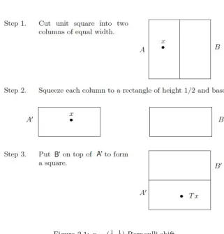
Figure 2.1: p= (1₂,1₂)-Bernoulli shift

In the same manner, we can construct a 1₃,1₃,1₃-Bernoulli shift using the

Baker’s Transformation. If we compute the entropies of a 1₂,1₂-Bernoulli shift and a

1 3,

1 3,

1 3

-Bernoulli shift, we will notice that the entropies are not the same; consequently,

these Bernoulli shifts are not isomorphic. In fact, we can state that two Bernoulli shifts

with the same entropy are isomorphic and this was proved by Ornstein in 1970.

Example 2.3.2. Markov Shifts. Now, consider a finite scheme(X0, p)and the infinite

product space X = XZ

0 with a Bernoulli shift S. Let M = [mij] be an l×l stochastic

matrix, i.e., mij ≥0, l

Σ

j=1mij = 1 for 1

≤i, j ≤l, and m= (m1, ..., ml) be a probability

distribution such that Σl

i=1mimij =mj for 1

≤ j ≤ l. Each mij indicates the transition

probability from the state ai to the state aj and the row vector of m is fixed by M in the

sense that mM =m. We always assume thatmi>0for everyi= 1, ..., l. Now we define

µ0([ai0· · ·ain]) =mi0mi0i1· · ·min−1in.

µ0 is uniquely extended to a measure µon X which isS-invariant. The shift S

is called an (M, m)-Markov shift.

To compute the entropy of an (M, m)-Markov shift S consider a partition A= {[x0 =a1], ...,[x0=al]} ∈ P(X), which satisfies

∞

∨

n=−∞S

n_A˜ _{=X. As the example before,}

H

n−1

∨

k=0S −k_A

=− X

x0,...,xn−1∈X0

µ([x0· · ·xn−1]) logµ([x0· · ·xn−1])

=−

l

X

i0,...,in−1

mi0mi0i1· · ·min−2in−1logmi0mi0i1· · ·min−2in−1

=−

l

X

i0=1

mi0logmi0 −(n−1)

l

X

i,j=1

mimijlogmij

since

l

P

i=1

mimij =mj and l

P

j=1

mij = 1 for 1≤i, j ≤l. By dividing nand letting n→ ∞

we get

H(S) =−

l

X

i,j=1

Chapter 3

Relative Entropy and

Kullback-Leibler Information

3.1

Introduction

In chapter 1, we define mutual information as a measure of the amount of information one random variable contains about the other one. We also observed the

self-information of a random variable becomes the entropy of the same random variable.

A more general case of a mutual information is the relative entropy. Therelative entropy

is a measure of the distance between two probability distributions. Here we will define

the relative entropy H(p|q) for two finite probability distributions p and q and provide

certain properties and an application in the field of statistics. In addition, we define the

relative entropy for two distributionspandqof a continuous random variable and extend

the concept to an arbitrary pair of probability measures.

3.2

Discrete Relative Entropy and Its Properties

Definition 3.2.1. Let p, q ∈ ∆n. The relative entropy H(p|q) of p w.r.t. (with respect

to) q is given by

H(p|q) =

n

X

j=1

pjlog

pj

qj

.

As before, we use the convention that 0 log0₀ = 0 and 0 log_q0

j = 0. But if pj > 0 and

The notion of the relative entropy as distance of two probability distributions is

not a metric because it does not satisfy the triangle inequality or the symmetry property

of a metric. Notwithstanding, the relative entropy H(p|q) is a measure of the

ineffi-ciency assumption [Kul97]. The next example illustrates that the relative entropy is not

symmetric.

Example 3.2.1. Let the random variable X ={0,1} and suppose that p and qare two probability distributions of X. Letp= (1−p, p), and letq= (1−q, q). Now, we have

H2(p|q) = (1−p) log

1−p

1−q +plog p q

and

H2(q|p) = (1−q) log

1−q

1−p+qlog q p.

Notice if p = q, then H2(p|q) = H2(q|p) = 0. Now suppose that p = 1₄ and

q = 1₈. Then

H2(p|q) = (1−

1 4) log

1−1 4

1−1₈ + 1 4log

1 4 1 8

= 3 4log

6 7+

1

4 = 0.0832bit.

but

H2(q|p) = (1−

1 8) log

1−1 8

1−1₄ + 1 8log

1 8 1 4

= 7 8log

7 6−

1

8 = 0.0696bit.

Thus, H2(p|q)6=H2(q|p).

In the next definition, we consider p(x, y) and q(x, y) be two joint probability

distributions for the pair of random variables (X, Y) and p(x) be the probability

distri-bution for X.

Definition 3.2.2. Given the joint probabilitiesp(x, y)andq(x, y), the conditional relative entropy is defined as

H(p(y|x)|q(y|x)) =X

x

p(x)X

y

p(y|x) logp(y|x) q(y|x).

The conditional relative entropy is the average of the relative entropies between

the conditional probability distributions p(y|x) and q(y|x) averaged over the probability

distribution p(x). Now, we define the relative entropy between two joint probability

distributions on (X, Y) in terms of a sum of relative entropy and a conditional relative

Theorem 3.2.1. The relative entropy between two joint probability distributions p(x, y)

and q(x, y) on(X, Y) is given by

H(p(x, y)|q(x, y)) =H(p(x)|q(x)) +H(p(y|x)|q(y|x)).

Proof. Observe that H(p(x, y)|q(x, y)) = X

x∈X

X

y∈Y

p(x, y) logp(x, y) q(x, y)

= X

x∈X

X

y∈Y

p(x, y) logp(x)·p(y|x) q(x)·q(y|x)

= X

x∈X

X

y∈Y

p(x, y) logp(x) q(x) +

X

x∈X

X

y∈Y

p(x, y) logp(y|x) q(y|x)

= X

y∈Y,x∈X

p(x, y) logp(x, y) + X

y∈Y,x∈X

p(x, y) logp(y)

=H(p(x)|q(x)) +H(p(y|x)|q(y|x)).

To prove some fundamental properties in information theory, we have used the

concept of convexity. In this chapter, we will define convexity and state the Jensen’s

inequality. Then, we will use these concepts to show some properties of the relative

entropy.

Definition 3.2.3. A functionϕ: (a, b)→Ris convex if ϕ

n

X

i=1

λixi

! ≤

n

X

i=1

λiϕ(xi)

for all xi ∈ (a, b) and λi ∈ [0,1] with Pni=1λi = 1. The equality holds when xi =x for

some x∈(a, b) and all i withλi>0. We also say that ϕ is strictly convex if

ϕ

n

X

i=1

λixi

! <

n

X

i=1

λiϕ(xi).

Definition 3.2.4. A function f is concave if −f is convex. A function is convex if it always lies bellow any chord. A function is concave if it always lies above any chord.

We also say a functionf is convex if the functionf has a second derivative that

Lemma 3.2.1. Jensen’s inequality. Let ϕ: (a, b) → _R be a convex function and let

f :X→(a, b) be a measurable function in L1 on a probability space (X,X, µ). Then

ϕ Z f(x)dµ(x) ≤ Z

ϕ(f(x))dµ(x).

and if ϕ is strictly convex, then

ϕ Z

f(x)dµ(x)

< Z

ϕ(f(x))dµ(x)

unless f(x) =t for µ-almost everyx∈X for some fixed t∈(a, b).

In particular, If f is a convex function and X is a random variable,

Ef(X)≥f(EX).

The equality holds true whenever X=EX with probability 1, that is,X is constant.

Lemma 3.2.2. (Log-Sum Inequality) Letpi, qi >0 for 1≤i≤n. Then n

X

i=1

pilog

pi qi ≥ n X i=1 pi ! log Pn

i=1pi

Pn

i=1qi

where equality holds if and only if pi

qi =constant.

Proof. First we claim that the function f(t) = tlogt is strictly convex. It is sufficient to show thatf00>0. Then, if we differentiate twice,f00(t) = 1_t >0 whent >0. By Jensen’s inequality, we also know that Pn

i=1αif(ti) ≥ f(

Pn

i=1αiti) with αi ≥ 0,

α1+· · ·+αn= 1. Now, letpi, qi >0 for 1≤i≤n. Then we have

n

X

i=1

pilog

pi qi = n X i=1

qif

pi qi = n X i=1 qi n X i=1 qi Pn

i=1qi

f pi qi ≥ n X i=1

qif n

X

i=1

qi

Pn

i=1qi

·pi qi ! = n X i=1

qif

Pn

i=1pi

Pn

i=1qi

=

n

X

i=1

qi·

Pn

i=1pi

Pn

i=1qi

log Pn

i=1pi

Pn

i=1qi

=

n

X

i=1

pilog

Pn

i=1pi

Pn

i=1qi

.

We next establish some important properties of the relative entropy by using

lemma 3.2.2.

Theorem 3.2.2. Let p andq be two probability distributions of the random variable X. Then we have

i. Nonnegativity. H(p|q)≥0, and H(p|q) = 0 if and only if p = q.

ii. Convexity. Let p1, p2, q1, q2 be probability distributions of the random variableX.

Then, for α∈[0,1], we have

H(αp1+ (1−α)p2|αq1+ (1−α)q2)≤αH(p1|q1) + (1−α)H(p2|q2).

iii. Partition Inequality. If A={A1, ..., Ak} is a partition of X. That is,∪ki=1Ai=

X, and Ai∩Aj =∅ whenever i6=j. Define

pA(i) =

X

x∈Ai

p(x), i= 1, ..., k,

qA(i) =

X

x∈Ai

q(x), i= 1, ..., k,

then

H(p|q)≥H(pA|qA),

where equality holds if and only if p(x) =q(x) for each x∈Ai.

Proof.

(i.) By definition, we have

H(p|q) = X

x∈X

p(x) logp(x) q(x)

≥ X

x∈X

p(x) !

log P

x∈Xp(x)

P

x∈Xq(x)

, by lemma 3.2.2,

= 1 log1 1

and it is clear that H(p|q) = 0 if and only ifp(x) =q(x) for allx∈X.

(ii.) Letp1, p2, q1, q2 be probability distributions of the random variable X and

α∈[0,1]. Then

H(αp1+ (1−α)p2|αq1+ (1−α)q2)

= X

x∈X

(αp1(x) + (1−α)p2(x)) log

αp1(x) + (1−α)p2(x)

αq1(x) + (1−α)q2(x)

= X

x∈X

αp1(x) log

αp1(x) + (1−α)p2(x)

αq1(x) + (1−α)q2(x)

+X

x∈X

(1−α)p2(x) log

αp1(x) + (1−α)p2(x)

αq1(x) + (1−α)q2(x)

≤ X

x∈X

αp1(x) log

αp1(x)

αq1(x)

+X

x∈X

(1−α)p2(x) log

(1−α)p2(x)

(1−α)q2(x)

, by lemma 3.2.2,

=αX

x∈X

p1(x) log

p1(x)

q1(x)

+ (1−α)X

x∈X

p2(x) log

p2(x)

q2(x)

=αH(p1|q1) + (1−α)H(p2|q2).

(iii.) LetA={A1, ..., Ak}be a partition of X. Then

H(p|q) =X

x∈X

p(x) logp(x) q(x) = k X i=1 X

x∈Ai

p(x) logp(x) q(x) ≥ k X i=1   X

x∈Ai

p(x) 

log P

x∈Aip(x)

P

x∈Aiq(x)

=

k

X

i=1

pA(i) log

pA(i)

qA(i)

, by hypothesis,

=H(pA|qA).

One of the applications that involves the relative entropy is a statistical

H0 :p= (p(a1), ..., p(an))

H1 :q= (q(a1), ..., q(an)),

and we have to decide which one is true depending on the samples of size k, where

p, q ∈ ∆n and X0 = {a1, ..., an}. We need to find a set A ⊂ X0k, so that, for a sample

(x1, ..., xk)∈A, thenH0 is accepted; otherwiseH1 is accepted. Here, for some ∈(0,1),

type 1 error probability P(A) satisfies

X

(x1,...,xk)∈A

k

Y

j=1

p(xj) =P(A)≤

and type 2 error probabilityQ(A) is given by

X

(x1,...,xk)∈/A

k

Y

j=1

q(xj) = 1−Q(A) =Q(Ac),

which should be minimized. Thus, for any ∈(0,1) and the sample size k≥1 let

β(k, ) = min{Q(Ac) :P(Ac)>1−, A⊂Xk}.

Then we claim that

lim

k→∞

1

kβ(k, ) =−

n

X

j=1

p(aj) log

p(aj)

q(aj)

=−H(p|q).

It follows from the claim that we can minimize the probability Q(Ac) with

respect to P(Ac) by calculating the relative entropy−H(p|q), the negative entropy of p

with respect to q. A proof of this claim is found in [Kak99]. Next, we define the relative

entropy given a continuous random variable.

3.3

Continuous Entropy and Relative Entropy

Definition 3.3.1. Let X be a random variable with cumulative distribution function

F(x) =P(X ≤x). If F(x) is continuous, the random variable is said to be continuous. Let f(x) =F0(x) when the derivative is defined. If

Z

R

f(x) is called the probability density function forX. The set where f(x)>0 is called the support set of X. Now, we define the expected value of X by

E(X) = Z

R

xf(x)dx.

Definition 3.3.2. The entropy H(X) of a continuous random variable X with density

f(x) is defined as

H(X) =− Z

S

f(x) logf(x)dx,

where S is the support set of the random variable, and given that the integral exists.

Now, we define the relative entropy of a continuous random variableX and show

some of its properties.

Definition 3.3.3. The relative entropy H(f|g) between two densities f and g is defined by

H(f|g) = Z

flogf g

Note thatH(f|g) is finite only if the support set of f is contained in the support set of g.

In chapter 1, the discrete entropy is maximized when a set of events are equally

likely, that is, uniformly distributed. In the continuous case, the result is similar and it

is shown in the next example.

Example 3.3.1. (Uniform Distribution) Let f be the probability density function on

(a, b) given by

f(x) =   

 

1

b−a, ifa < x < b 0, otherwise

Let us find the entropy of a random variable X with a uniform density functionf. Then,

H(X) =− Z

(a,b)

f(x) logf(x)dx

=− Z

(a,b)

1 b−alog

1 (b−a) dx

= 1

b−alog(b−a) Z

(a,b)

dx

Now, assume thatf(x) is a probability density function on(a, b) andg(x) is the uniform density function on (a, b). Then,

H(f|g) = Z

(a,b)

f(x) logf(x) g(x) dx

= Z

(a,b)

f(x)(logf(x)−logg(x))dx

=−H(X)−log 1 (b−a)

Z

(a,b)

f(x)dx

=−H(x) + log(b−a)≥0.

First we notice that, as the discrete case, the relative entropyH(f|g)≥0. Also, this example provides us with an upper bound for a probability density function on the interval (a, b), i.e., H(X)≤log(b−a).

We also find the relative entropy between two normal and exponential

probabil-ity densprobabil-ity functions on a random variable X.

Example 3.3.2. (Normal Distribution)A random variable X is normally distributed with parameters µand σ2 if the probability density function f(x) is defined by

f(x) = √ 1 2πσ2e

−(x−µ)2_/2σ2

, −∞< x <∞.

Suppose that f and g are normally distributed with parameters µ1, σ21 and µ2 ,

σ2₂, respectively. Then we have

H(f|g) = Z

f(x) logf(x) g(x) dx

= Z

f(x) log

1

q

2πσ2 1

e−(x−µ1)2/2σ12

1

q

2πσ2 2

e−(x−µ2)2/2σ22

dx

= Z

f(x) log

σ₂2 σ₁2

1/2 dx+

Z f(x)

−(x−µ1)

2

2σ2₁ +

(x−µ2)2

2σ₂2

dx

= 1 2log

σ2₂ σ2₁

Z

f(x)dx− Z

f(x)(x−µ1)

2

2σ2₁ dx+ Z

f(x)(x−µ2)

2

2σ2₂ dx

= 1 2log

σ2₂ σ2₁ ·1−

1

2σ2₁V ar(X) + 1 2σ2₂

Z

= 1 2log

σ2₂ σ2₁ −

1 2 +

1 2σ₂2 ·

Z

f(x)(x−µ1)2dx

+ 1

2σ2₂ ·2(µ1−µ2) Z

f(x)(x−µ1)dx+

1

2σ₂2 ·(µ1−µ2)

2

Z

f(x)dx

= 1 2log

σ2₂ σ2₁ −

1 2 +

1

2σ₂2(V ar(X) + 2(µ1−µ2)·(E(X)−µ1) + (µ1−µ2)

2₎ = 1 2 logσ 2 2

σ2₁ +

σ₁2+ (µ1−µ2)2

σ₂2 −1

,

where the variance V ar(X) =E[(X−µ1)2] =

R

f(x)(x−µ1)2 =σ21 .

Example 3.3.3. (Exponential Distribution) A continuous random variableX is said to be exponentially distributed for λ >0 if the density function is defined as

f(x) =     

λe−λx, if x≥0 0, if x <0.

The entropyH(X)with exponentially density functionf is calculated as follows:

H(X) =− Z

f(x) logf(x)dx

=− Z

λe−λxlogλe−λxdx

=− Z

λe−λx[logλ+ loge−λx]dx

=− Z

λe−λxlogλ dx− Z

λe−λx(−λx)dx

=−logλ Z

λe−λxdx+λ Z

xλe−λxdx

= logλ·1 +λ·E(X)

=−logλ+ 1.

We now find the relative entropy of two exponentially distributed functions f

with parameter λ1 and g with parameter λ2.

H(f|g) = Z

f(x) logf(x) g(x) dx

= Z

= Z

f(x) logf(x)dx− Z

f(x) logg(x)dx

=−H(X)− Z

λ1e−λ1x[logλ2+ loge−λ2x]dx

=−(−logλ1+ 1)−logλ2

Z

λ1e−λ1xdx+

Z

λ2xλ1e−λ1xdx

= logλ1−1−logλ2·1 +λ2

Z

xλ1e−λ1xdx

= logλ1−1−logλ2+λ2·E(X)

= logλ1 λ2

+λ2 λ1

−1,

where E(X) =R

xλ1e−λ1xdx= _λ1₁.

Now, we extend the definition of the relative entropy between two probability

measures.

Definition 3.3.4. Let (X,X) be a measurable space. Let P(X) denote the set of all probability measures onXandP(Y)denote set of all finiteY-measurable partitions ofX, where Y is a σ-subalgebra of X. Let µ, ν ∈ P(X). Then, the relative entropy of µ with respect to ν relative to Yis defined by

HY(µ|ν) = sup

( X

A∈A

µ(A) logµ(A)

ν(A) :A∈P(Y) )

.

If Y= X, then we write HX(µ|ν) = H(µ|ν) and call it the relative entropy of

µ with respect to ν. Note that the relative entropy is defined for any pair of probability measures.

If µν,µ is absolutely continuous with respect to ν, relative entropy has an

integral form. That is,

H(µ|ν) = Z

X

dµ dν log

dµ dν

dν =

Z

X

logdµ dνdµ,

and if µ is not absolutely continuous with respect toν, then H(µ|ν) =∞.

Definition 3.3.5. (Kullback-Leibler information) Let ξ and η be real random vari-ables on (X,X, µ), so that they have probability distributions µξ and µη given by

respectively and B is the Borel σ-algebra of R. Suppose that µξ and µη are absolutely

continuous with respect to the Lebesgue measure dt of R, so that we have the probability

density functions f and g, respectively given by

f = dµξ

dt , g= dµη

dt ∈L

1₍

R) =L1(R, dt).

Then the Kullback-Leibler information between ξ and µis given by

I(ξ|µ) = Z

R

(f(t) logf(t)−f(t) logg(t))dt.

Observe that given the definition above and the integral form of H(µξ|µη), we

have

I(ξ|µ) = Z

R

(f(t) logf(t)−f(t) logg(t))dt

= Z

R

f(t) logf(t) g(t) dt

= Z

R dµξ

dt log

dµξ

dt dµη

dt

dt

= Z

R dµξ

dµη

logdµξ dµη

dµη

=H(µξ|µη).

Therefore, the relative entropy, in general, is interpreted as theKullback-Leibler

information.

3.4

Birkhoff Pointwise Ergodic Theorem

So far, we have introduced a way of measuring the amount of information by

calculating the entropy of a system. Now, we want a way of studying the long term

average behavior of a system that evolves over time. In this section, we state and show

the proof of a main theorem found inAbstract Methods in Information Theoryby [Kak99]. This theorem will help us to describe that long term average behavior. We say that the

collection of all states of the system form a space X, and the evolution is represented by

a transformation S:X→X. Since we want S to preserve the basic structure on X, we

Definition 3.4.1. Let S be a measure preserving transformation on a probability space

(X,X, µ). The map S is said to be ergodic if for every measurable set A satisfying

S−1A=A, we haveµ(A) = 0 or µ(A) = 1.

The next theorem is a generalization of the Strong Law of Large Numbers. That

is, if we have a sequence X1, X2, ... of independent and identically distributed random

variables with the expectation E(Xi) =µ, then lim n→∞

1 n

n

P

i=1

Xi=µ almost surely. We say

that an event isalmost surely if the event occurs with probability one even if it does not contain all possible outcomes. The outcome or set of outcomes not contained in the event

has probability zero [Dur05].

Theorem 3.4.1. Birkhoff Pointwise Ergodic TheoremLet(X,X, µ)be a probability space and S : X → X a measure preserving transformation and f ∈ L1(X, µ). Then, there exists a unique fS ∈L1(X, µ) such that

lim

n→∞

1 n

n−1

X

i=0

f(Six) =fS

exits a.e., is S-invariant and R

Xf dµ=

R

XfS dµ. If moreover S is ergodic, then fS is a

constant a.e. and fS =

R

Xf dµ.

Proof. Let f ∈ L1(X, µ) and without loss of generality consider f ≥0. Define fn(x) =f(x) +· · ·+f(Sn−1x), ¯f = lim

n→∞sup

fn

n, andf = limn→∞inf

fn

n. Then ¯f andf are S-invariant. Observe that

f(Sx) = lim

n→∞inf

fn(Sx)

n

= lim

n→∞inf

fn+1(x)

n+ 1 · n+ 1

n − f(x)

n

= lim

n→∞inf

fn+1(x)

n+ 1 .

We show ¯f is S invariant in the same manner. We next show that fS exists, is

integrable and S-invariant. It suffices to show that

Z

X

¯ f dµ≤

Z

X

f dµ≤ Z

X

f dµ.

Since ¯f −f ≥0, this would imply that ¯f =f =fS a.e.. Let M >0 and > 0

¯

fM(x) = min{f¯(x), M}, x∈X.

Define n(x) to be the least integern≥1 such that

¯ fM(x)≤

fn(x)

n += 1 n

n−1

X

j=0

f(Sjx) +, x∈X.

Note thatn(x) is finite for eachx∈X. Since ¯f and ¯fM(x) areS-invariant, we have

n(x) ¯fM(x)≤n(x)[(

fn(x)

n(x) ¯

fM)(x) +] = n(x)−1

X

j=0

f(Sjx) +n(x), x∈X. (3.1)

Choose a large enough N ≥1 such that

µ(A)<

M with A={x∈X:n(x)> N}.

Now we define ˜f and ˜nby

˜ f(x) =

  

 

f(x), x /∈A

0, x∈A

, ˜n(x) =   

 

n(x), x /∈A

1, x∈A .

Then we see that for all x∈X

˜

n(x)≤N, by definition,

˜

n(x)−1

X

j=0

¯

fM(Sjx)≤

˜

n(x)−1

X

j=0

˜

f(Sjx) + ˜n(x), (3.2)

by (3.1) and S-invariance of ¯fM, and that

Z

X

˜ f dµ=

Z

Ac

f dµ+ Z A ˜ f dµ ≤ Z Ac

f dµ+ Z

A

f dµ+ Z A M dµ = Z X

f dµ+ Z

A

M dµ≤ Z

X

f dµ+.

Furthermore, find an integerL≤1 so that N M_L < and define a sequence{nk(x)}∞k=0 for

each x∈X by

n0(x) = 0, nk(x) =nk−1(x) + ˜n(Snk(x)x), k≥1.

Then it holds that for x∈X

L−1

X

j=0

¯

fM(Sjx) = k(x)

X

k=1

nk(x)−1

X

j=nk−1(x)

¯

fM(Sjx) + L−1

X

j=nk(x)(x)

¯

fM(Sjx),

where k(x) is the largest integerk≥1 such that nk(x)≤L−1. Applying (3.2) to each

of the k(x) terms and estimating byM the lastL−nk(x)(x) terms, we have

L−1

X

j=0

¯

fM(Sjx) = k(x)

X

k=1

nk(x)−1

X

j=nk−1(x)

¯

fM(Sjx) + L−1

X

j=nk(x)(x)

¯ fM(Sjx)

≤

k(x)

X

k=1





nk(x)−1

X

j=nk−1(x)

˜

f(Sjx) + (nk(x)−nk−1(x))



+ (L−n_k(x)(x))M

≤

L−1

X

j=1

˜

f(Sjx) +L+ (N−1)M

since ˜f ≥ 0, ¯fM ≤ M and L−nk(x)(x) ≤ N −1. If we integrate both sides on X and

divide by L, then we get

Z

X

¯

fM dµ≤

Z

X

˜

f dµ++(N −1)M L ≤

Z

X

f dµ+ 3

by the S-invariance of µ, (3.3) and N M_L < . Thus, letting → 0 and M → ∞ give

the inequality R _¯

f dµ≤R

Xf dµ. The other inequality

R

f dµ≤R

Xf dµ can be obtained

similarly. Hence, ¯f =f =fS a.e., andfS isS-invariant. IfSis ergodic, thenS-invariance

of fS implies thatfS is a constanta.e and

fS(x) =

Z

X

fS(y)dµ(y) =

Z

X

Chapter 4

Conclusion

In this thesis, we presented some topics in information theory and developed

some examples as applications in different fields of study. As we developed this topics, we

unraveled the importance of measure theoretic and functional analysis methods in order

to define and characterize some of the properties in information theory.

In chapter one, to describe the amount of information of a source, we developed

the theory of entropy. Specifically, we defined Shannon entropy for finite scheme and some of its properties. We showed some examples by finding the entropy of Bernoulli,

Geometric, and Poisson probability distributions. We also defined the entropy function

and provided a useful inequality in coding theory. In next chapter, we defined a dynamical

system and a measurable partition to define the Kolmogorov-Sinai entropy. Next, we stated and proved the Kolmogorov-Sinai theorem. We defined and showed that Bernoulli Shifts with the same entropy are isomorphic. To finish, we calculated the entropy of

Markov Shifts by also usingKolmogorov-Sinai theorem.

In the last chapter, we do not only define relative entropy for finite probability

distributions and probability density functions, but also we extended this definition to

an arbitrary pair of probability measures and then defined Kullback-Leibler information. We proved some essential properties of the relative entropy and provided an application

in statistical hypothesis testing. Furthermore, we calculated the relative entropy for

the Uniform, Normal, and Exponential distributions. Finally, we briefly developed the

Bibliography

[Ash67] Robert Ash. Information Theory. Interscience, New York, NY, 1967.

[CT06] Thomas M. Cover and Joy A. Thomas. Elements Of Information Theory. Wiley Interscience, Hoboken, NJ, 2006.

[Dur05] Richard Durrett. Probability: Theory and Examples. Curt Hinrichs, Belmont, CA, 2005.

[Kak99] Yuichiro Kakihara. Abstract Methods In Information Theory. Word Scientific, River Edge, NJ, 1999.

[Kul97] Solomon Kullback. Information Theory And Statistics. Dover, Mineola, New York, 1997.

[Pie80] John R. Pierce. An Introduction to Information Theory: Symbols, Signals and Noise. Dover, New York, NY, 1980.

[Rom92] Steven Roman. Coding and Information Theory. Springer-Verlag, New York, NY, 1992.

[Ros07] Sheldon M. Ross. Introduction to Probability Models. Academic Press, New York, NY, 2007.

[Shr04] Steven E. Shreve. Stochastic Calculus for Finance II: Continuous-Time Models. Springer, New York, NY, 2004.