The Linear Cutwidth and Cyclic Cutwidth of Complete n-Partite Graphs

(1)

Electronic Theses, Projects, and Dissertations Office of Graduate Studies

6-2014

The Linear Cutwidth and Cyclic Cutwidth of Complete n-Partite

Graphs

Stephanie A. Creswell

California State University - San Bernardino

Follow this and additional works at: https://scholarworks.lib.csusb.edu/etd

Part of the Discrete Mathematics and Combinatorics Commons

Recommended Citation Recommended Citation

Creswell, Stephanie A., "The Linear Cutwidth and Cyclic Cutwidth of Complete n-Partite Graphs" (2014). Electronic Theses, Projects, and Dissertations. 34.

https://scholarworks.lib.csusb.edu/etd/34

(2)

A Thesis

Presented to the

Faculty of

California State University,

San Bernardino

In Partial Fulfillment

of the Requirements for the Degree

Master of Arts

in

Mathematics

by

Stephanie Anne Creswell

(3)

A Thesis

Presented to the

Faculty of

California State University,

San Bernardino

by

Stephanie Anne Creswell

June 2014

Approved by:

Joseph Chavez, Committee Chair Date

Rolland Trapp, Committee Member

Min-Lin Lo, Committee Member

Peter Williams, Chair, Charles Stanton

Department of Mathematics Graduate Coordinator,

(4)

Abstract

The cutwidth of different graphs is a topic that has been extensively studied.

The basis of this paper is the cutwidth of complete n-partite graphs. While looking at

the cutwidth of completen-partite graphs, we strictly consider the linear embedding and

cyclic embedding. The relationship between the linear cutwidth and the cyclic cutwidth

is discussed and used throughout multiple proofs of different cases for the cyclic cutwidth.

All the known cases for the linear and cyclic cutwidth of complete bipartite, complete

tripartite, and complete n-partite graphs are highlighted.

The main focus of this paper is to expand on the cyclic cutwidth of complete

tripartite graphs. Using the relationship of the linear cutwidth and cyclic cutwidth of

any graph, we find a lower bound and an upper bound for the cyclic cutwidth of complete

tripartite graphKr,r,pr wherer is odd and pis a natural number. Throughout this proof

there are two cases that develop, peven andpodd. Within each case we have to consider

the cuts of multiple regions to find the maximum cut of the cyclic embedding. Once all

regions within each case are considered, we discover that the upper and lower bounds

are equivalent. This discovery of the cyclic cutwidth of complete tripartite graph Kr,r,pr

wherer is odd andp is a natural number results in getting one step closer to finding the

(5)

Acknowledgements

First I want to give a generous thank you to Dr. Joseph Chavez for all of his

guidance and encouragement with the research and development of this paper. Secondly,

I’d like to thank Dr. Rolland Trapp and Dr. Min-Lin Lo for their feedback and support

throughout this process. I also would like to give a special thank you Dr. Chavez, Dr.

Trapp and Dr. McMurran for their support, encouragement, and belief in me throughout

my whole college education. In addition to their efforts in making me a better student,

they challenged me beyond the classroom exposing me to experiences I never would have

challenged myself to. It has been an honor to work with these professors and they have

inspired me to be a better educator with my own students.

I’d also like to thank my classmates Trinity, Jeff, Matt, and Joe for all of their

support and encouragement throughout each class. It has been a joy walking side by side

with all of them throughout this program. Above all I’d like to give a special thank you

to Trinity. I truly would have not made it through this program without her. She has

been by my side with every class and encouraged me through every challenge I faced.

Lastly I’d like to thank my family for always supporting me in my studies. My

parents and my in-laws have encouraged me and been so understanding with the

com-mitment to this program. Most importantly, the largest thank you goes to my husband

(6)

List of Figures

1.1 Complete Bipartite GraphK3,4 and Complete Tripartite Graph K2,3,4 . . 2

1.2 Linear Embedding of Complete Tripartite GraphK2,3,4 . . . 3

1.3 Cyclic Embedding of Complete Bipartite GraphK3,4 . . . 4

1.4 Cut of Each Region of GraphK3,5 Within a Linear and Cyclic Embedding 5 1.5 Cut of Each Region of GraphK3,5 Within a Linear Embedding . . . 5

1.6 Tripartite Arrangement of GraphK3,5,7 . . . 12

1.7 Cyclic Arrangement of GraphG . . . 13

1.8 Linear Arrangement of GraphG . . . 14

1.9 Vertex Arrangement forK5,5,5. . . 18

1.10 Top Black Vertex Edge Contribution toα1 of K5,5,5 . . . 19

1.11 Remaining r−1 Black Vertices Arrangement of K5,5,5 . . . 20

1.12 First Clockwise Black Vertex Edge Contribution toα1 of K5,5,5 . . . 21

1.13 Second Clockwise Black Vertex Edge Contribution toα1 ofK5,5,5 . . . 21

1.14 First Clockwise Grey Vertex Edge Contribution toα1 of K5,5,5 . . . 23

1.15 Second Clockwise Grey Vertex Edge Contribution to α1 of K5,5,5 . . . 23

1.16 First Counter-Clockwise Grey Vertex Edge Contribution to α1 ofK5,5,5 . 25 2.1 Vertex Arrangement forKr,r,pr . . . 31

2.2 Regionsα1 and α2 . . . 32

2.3 Diameters ofK5,5,20 . . . 33

2.5 Remainingr−1 Black Vertices Arrangement of K5,5,20. . . 35

2.7 Second Clockwise Black Vertex Edge Contribution toα1 ofK5,5,20 . . . . 36

2.8 Botttom Grey Vertex Edge Contribution toα1 ofK5,5,20 . . . 38

2.9 Grey vertex Placement ofK5,5,20 . . . 39

2.11 Second Clockwise Grey Vertex Edge Contribution to α1 of K5,5,20. . . 40

2.12 Regions α1 and α2 . . . 42

2.13 Regionα2 of K3,3,24 . . . 43

2.14 First Clockwise White Vertex Edge Contribution toα2 of K3,3,24 . . . 43

2.15 Second and Third Clockwise White Vertex Edge Contribution toα2ofK3,3,24 44

(8)

2.17 Diameters Contributing to The Cut of Regionα2 of K3,3,24 . . . 47

2.18 Regions α1,α2,α3, andα4 . . . 50

2.20 Remaining r−1 Black Vertices Arrangement of K3,3,21. . . 52

2.23 Regions α1,α2,α3, andα4 . . . 57

2.24 Rotation of Cyclic Embedding for α2 ofK3,3,21 . . . 57

2.25 Top Grey Vertex Edge Contribution to α2 ofK3,3,21 . . . 58

2.26 Remaining r−1 Black Vertices Arrangement of K3,3,21. . . 59

2.29 Regions α1,α2,α3, andα4 . . . 63

2.30 Regionα3 of K3,3,21 Rotated . . . 64

2.31 Top White Vertex Edge Contribution to α3 ofK3,3,21. . . 65

2.32 Top Set of White Vertices Edge Contribution toα3 of K3,3,21 . . . 65

2.33 First Set of White Vertices Clockwise Top Set Edge Contribution to α3 of K3,3,21 . . . 66

2.34 Black Vertex in Set Opposite Top White Set Edge Contribution to α3 of K3,3,21 . . . 68

2.35 First Black Vertex Clockwise Top White Vertex Edge Contribution to α3 ofK3,3,21 . . . 69

2.36 First Black Vertex Counter-Clockwise Top White Vertex Edge Contribu-tion toα3 of K3,3,21 . . . 70

2.37 Regions α1,α2,α3, andα4 . . . 72

2.38 Regionα4 of K3,3,21 Rotated . . . 73

2.39 Top White Vertex Edge Contribution to α4 ofK3,3,21. . . 73

2.40 Top Set of White Vertices Edge Contribution toα3 of K3,3,21 . . . 74

2.41 First Set of White Vertices Clockwise Top Set Edge Contribution to α4 of K3,3,21 . . . 75

2.42 First Black Vertex Clockwise Top White Vertex Edge Contribution to α4 ofK3,3,21 . . . 77

(9)

Chapter 1

Background

In this chapter we will introduce complete n-partite graphs and two different

ways these graphs can be arranged. Within the linear embedding we will discuss the

linear cutwidth of complete bipartite and complete tripartite graphs. We will only

dis-cuss the proofs involving the linear embedding and linear cutwidth of complete bipartite

graphs, since the proofs for the complete tripartite graphs are similar. Within the cyclic

embedding we will discuss certain cases discovered for the cyclic cutwidth of complete

bipartite graphs and complete tripartite graphs. We will only discuss the proof of the

lower bound for the cyclic cutwidth of any complete tripartite graph and the proof of the

cyclic cutwidth for graphKr,r,r when r is odd since they relate to the proof in chapter 2.

1.1

Complete n-Partite Graphs

A graph consists of vertices and edges, where one edge connects two vertices.

Visually, vertices are represented by dots and edges are represented by lines. Although

there are many different types of graphs, the focus of this paper will be on complete

n-partite graphs, denoted Km1,m2,...,mn. A complete n-partite graph is defined to have

n different groups of vertices V1, V2, ..., Vn, where |V1|=m1,|V2|=m2, ...,|Vn|=mn, such

that no vertex within group Vk,k= 1,2, ..., n, connects to any other vertex within group

Vk, but is connected to every vertex not in groupVk. Notemk≥1 and n≥2.

Many examples and proofs within this paper will consist of complete bipartite

(10)

n = 2. A complete tripartite graph is a complete n-partite graph where n= 3. In this

paper a complete bipartite graph will be represented by Km,n and complete tripartite

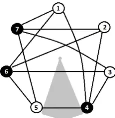
graph will be represented by Kr,s,t. Below Figure 1.1 shows examples of a complete

bipartite graph K3,4 and a complete tripartite graph K2,3,4.

Figure 1.1: Complete Bipartite GraphK3,4 and Complete Tripartite GraphK2,3,4

Vertices of an n-partite graph can be arranged in many different embeddings.

This paper will focus on a linear embedding and a cyclic embedding.

1.2

Linear Embedding

A linear embedding consists of an arrangement of all the vertices in a single line.

Figure 1.2 is the linear embedding of the complete tripartite graph K2,3,4 from Figure

1.1. The vertices that were connected in the non-linear representation of the graph will

(11)

Figure 1.2: Linear Embedding of Complete Tripartite GraphK2,3,4

A region in a linear embedding is the area between two adjacent vertices denoted

(v1, v2, ..., x−(v1 +v2+...+v(n−1))) for Km1,m2,...,mn, where x represents the number

of vertices to the left of the cut and vk represents the number of vertices left of the cut

from group Vk. Note that x−(v1+v2+...+v(n−1)) is the number of vertices to the left

of the cut from group Vn. In Figure 1.2 above, the region between vertices four and five

is shaded and is denoted as (1,1,2) wherex= 4.

1.3

Cyclic Embedding

A cyclic embedding consists of an arrangement of all the vertices in a circle.

Figure 1.3 is the cyclic embedding of the complete bipartite graph K3,4 from Figure 1.1.

The vertices that were connected in the non-cyclic representation of the graph will also

(12)

Figure 1.3: Cyclic Embedding of Complete Bipartite Graph K3,4

A region in a cyclic embedding is the area of a sector from the center of the circle

to two consecutive vertices on the edge of the circle. It is important to note that the cut

of a region (discussed later) is dependent on how many edges cross through the region.

Thus, no edge can pass through the center of the circle and must take a path through

adjacent regions to connect two vertices. Above in Figure 1.3, the region between vertices

four and five is shaded.

1.4

Cutwidth

The cut of a region is the number of edges that cross through the region between

two consecutive vertices. The region with the maximum cut within an embedding is the

region with the most edges crossing through it. Figure 1.4 shows the cut of each region for

one possible arrangement of the linear embedding and cyclic embedding of the complete

bipartite graph K3,5. The maximum cut of the arrangement for the linear embedding is

(13)

Figure 1.4: Cut of Each Region of Graph K3,5 Within a Linear and Cyclic Embedding

Note that these maximum cuts may not be the smallest maximum cut for the

linear embedding and the cyclic embedding for the graph K3,5. There may be another

arrangement within these embeddings that produce a smaller maximum cut. Figure 1.5

shows a second linear arrangement of the graph K3,5 that reduces the maximum cut.

Figure 1.5: Cut of Each Region of Graph K3,5 Within a Linear Embedding

The smallest maximum cut for all arrangements within each embedding is the

cutwidth of a graph. How to find the linear cutwidth and cyclic cutwidth for complete

(14)

1.5

Linear Cut

Recall a region in a linear embedding is the area between two adjacent vertices

denoted (v1, v2, ..., x−(v1+v2+...+v(n−1))) for Km1,m2,...,mn, where x represents the

number of vertices to the left of the cut and vk represents the number of vertices left

of the cut from group Vk. The cut of a region in a linear embedding can be found by

multiplying the number of vertices from each group left of the cut vi, i = 1,2, ..., n by

the number of vertices from each group right of the cut mj−nj, j = 1,2, ..., nand j6=i.

Thus, for a bipartite graph the cut of a region for a linear embedding can be found by

using the following.

cut(v1, x−v1) = v1(n−(x−v1)) + (x−v1)(m−v1)

Similarly for a tripartite graph the cut of a region for a linear embedding can

be found by using the following.

cut(v1, v2, x−(v1+v2)) = v1[(s−v2) + (t−(x−v1−v2))]

+v2[(r−v1) + (t−(x−v1−v2))]

+(x−v1−v2))[(r−v1) + (s−v2)]

1.6

Linear Cutwidth of Complete Bipartite Graphs

Before we look at the linear cutwidth of complete bipartite graphs we will look

at an arrangement of the linear embedding that minimizes the cut of each region.

Theorem 1 ([Bow04]). Let Km,n be a complete bipartite graph with two sets of vertices

V1 and V2, where |V1|= m and |V2|= n, and let m ≤ n. Let x represent the number of

vertices to the left of a region. Then the cut of each region of a linear embedding forKm,n

is minimized by placing 2x+m−n₄ vertices fromV1 to the left of the cut.

The following proof is a modified version of S. Bowles’ proof. [Bow04]

Proof. Letx be the number of vertices to the left of region, (v1, x−v1), within the linear

(15)

V1 to the left of this region. Thus, there arex−v1 vertices left of this region from setV2.

Note there are m−v1 vertices from set V1 and n−(x−v1) vertices from set V2 to the

right of this region. The cut of this region is as follows.

cut(v1, x−v1) = v1(n−(x−v1)) + (x−v1)(m−v1)

= v1n−v1x+v21+xm−v1x−v1m+v21

= 2v2₁+ (n−2x−m)v1+xm

Letf(v1) = 2v12+(n−2x−m)v1+xm. Notice thatf(v1) is a continuous function

of v1 ∈R, andf(v1) = cut(v1, x−v1) for 0≤v1 ≤m and v1 ∈Z. Note that the cut of

a region will vary depending on the arrangement of the linear embedding. The different

values for the cut of a region can be represented by a discrete function since we cannot

have an edge partially intersect a region. However, the function f(v1) is a continuous

representation of the possible cuts for a region and only the natural numbered solutions

can be considered. Since f(v1) is a positive quadratic function it has a minimum value.

If this minimum value is an integer, it represents the number of vertices from set V1 to

be are placed to the left of a region and will provide a minimum cut for that region. To

find this minimum value, we take the derivative off(v1) and set it equal to zero. Thus,

f0(v1) = 4v1+n−2x−m

0 = 4v1+n−2x−m

=⇒ v1 = m+2₄x−n

If v1 is not an integer, then f(v1) is a positive quadratic function, we get this

minimum value of f(v1) by rounding to the nearest whole number, denoted [v1]. Note

that this only happens since the graph is a positive quadratic. Thus, we are gaurenteed

(16)

the linear embedding of Km,n, it’s cut is minimized by placing

_m₊₂_x−n

4

vertices from

set V1 to the left of each region.

Now that the linear embedding of a complete bipartite graph can be arranged

such that the cut of each region is minimized, we will now look for the region of this

arrangement that contains the maximum cut.

Corollary 1 ([Bow04]). Let Km,n be a complete bipartite graph whose linear embedding

is arranged by Theorem 1. Then the maximum cut will occur when x= m+₂n for m+n

even and whenx= m+₂n−1 andx= m+₂n+1 for m+nodd. Also, the cuts to the left of the middle cut will be strictly increasing left to right and the cuts to the right of the middle cut will be strictly decreasing left to right.

Proof. Arrange the linear embedding by Theorem 1. Recall from the proof of Theorem 1, cut(v1, x−v1) = 2v12+ (n−2x−m)v1+xm. Also recallv1 = m+2₄x−n, minimizes the

cut of each region for the specific linear embedding. So consider the following.

cut(v1, x−v1) = 2v12+ (n−2x−m)v1+xm

= 2v2 1−4

(m+2x−n)v1

4 +xm

= 2v₁2−4v2₁+xm

= −2v2₁+xm

= −2

(m+2x−n) 4

2

+xm

= −1₈(m+ 2x−n)2+xm

(17)

for the minimized arrangement can be represented by a discrete function since we cannot

have an edge partially intersect a region. However, the function f(x) is a continuous

representation of the the cuts for each region for the minimized arrangement, and only

the natural numbered solutions can be considered. Since f(x) is a negative quadratic

function it has a maximum value. If this maximum value is an integer, it represents

the region where the maximum cut occurs for the minimized arrangement. To find this

maximum value, we take the derivative of f(x) and set it equal to zero. Thus,

f0(x) = −₄1(m+ 2x−n)2 +m

= m+₂n−x

0 = m+₂n−x

Observe that m+₂n −x > 0 when 1 < x < m+₂n and f(x) is increasing. Also

m+n

2 −x <0 when

m+n

2 < x < m+n andf(x) is decreasing. Thus, form+n even, the

maximum cut occurs at x = m+₂n. However, whenm+n is odd, m+₂n is not an integer

but is equally spaced between m+₂n−1 and m+₂n+1. Thus, the maximum cut will occur at

x= m+₂n−1 andx= m+₂n+1.

The proof of the linear cutwidth of a complete bipartite graph follows from

Theorem 1 and Corollary 1.

Theorem 2 ([Bow04]). Let Km,n be a complete bipartite graph. Then,

lcw(Km,n) =

  

mn

2 mn even

mn+1

2 mnodd

Proof. Let the complete bipartite graphKm,n be arranged by the algorithm in Theorem

1. From Theorem 1 and Corollary 1 the linear cutwidth of Km,n occurs when x = m+₂n

form+neven, and whenx= m+₂n−1 and x= m+₂n+1 form+n odd. To find the linear

(18)

Case 1: m+n even

Letm+nbe even, then the middle region of the linear embedding is atx= m+₂n.

By Theorem 1 placev1 =

₂_x₊m−n

4

vertices from setV1 to the left of the middle region.

Substituting m+₂n forx, we getv1 =

_m₊_n₊m−n

4

=_m

2

. Thus, v1 = m₂ when m is even

and v1 = m+1₂ when m is odd. Since m+n is even, we know that whenm is evenn is

also even, and when m is odd n is also odd. Therefore, the number of vertices, v2, from

set V2 to the left of the middle region are as follows.

v2=

  

x−m

2 =

n

2 forneven x− m+1

2 =

n−1

2 fornodd

Recall from section 1.5, the cut of a region can be found by cut(v1, x−v1) = v1(n−(x−v1)) + (x−v1)(m−v1). Consider the cut when mand nare both even.

cut m₂,n₂

= m₂ n₂ +m₂ n₂

= mn₂

Now consider the cut whenm and nare both odd.

cut m₂+1,n−₂1

= m₂+1n−₂1 +m−₂1n+1₂

= mn₂+1

Case 2: m+n odd

Let m+n be odd, then the middle regions of the linear embedding are at

x = m+₂n+1 and x = m+₂n−1. Without loss of generality, let’s consider the region where

x= m+₂n−1. By Theorem 1 placev1 =

₂_x₊m−n

4

vertices from setV1to the left of the

mid-dle region. Substituting m+₂n−1 for x, we get v1 =

_m₊n−1+m−n

4

= ₂m−1 4

=_m

2 − 1 4

.

Thus, v1 = m₂ when m is even and v1 = m−₂1 when m is odd. Since m+n is odd, we

know that when mis evennis odd, and whenmis oddnis even. Therefore, the number

(19)

v2=

  

x−m

2 =

n−1

2 fornodd x−m−1

2 =

n

2 forn even

Consider the cut whenm is even and nis odd.

cut m₂,n−₂1 = m₂ n+1₂ +m₂ n−₂1

= mn₂

Now consider the cut whenm is odd andn is even.

cut m−₂1,n₂ = m−₂1n₂ +m+1₂ n₂

= mn₂

Therefore,

lcw(Km,n) =

  

mn

2 mn even

mn+1

2 mnodd

1.7

Linear Cutwidth of Complete Tripartite Graphs

To find the linear cutwidth of a complete tripartite graph, the same structure

of proofs of a complete bipartite graph was followed. As a result Theorem 1, Corollary 1,

and Theorem 2 were developed. Note that the middle region consists of an arrangement

of rvertices from each setV1,V2, andV3, wherer represents the number of vertices from

the smallest set. The outer region is the arrangement of the remaining vertices and is

(20)

Figure 1.6: Tripartite Arrangement of GraphK3,5,7

Theorem 3 ([Bow04]). LetKr,s,t be a complete tripartite graph with three sets of vertices

V1,V2, andV3, where|V1|=r,|V2|=s, and|V3|=t, and letr≤s≤t. Also letxrepresent

the number of vertices to the left of a region. To minimize each cut of the linear embedding for Kr,s,t, the middle and outer sections of the graph are minimized independently. The

middle cuts are minimized by placing 2x+2r−s−t₆ vertices from A, 2x+2s−r−t₆ vertices from B, 2x+2t−r−s₆ vertices from C to the left of each cut. The outer sections are minimized according to Theorem 1 for complete bipartite graphs.

Corollary 2 ([Bow04]). Let Kr,s,t be a complete tripartite graph whose linear embedding

is arranged by Theorem 3. Then the maximum cut will occur when x= r+₂s+t forr+s+t

even and when x= r+s+₂t−1 and x= r+s+₂t+1 for r+s+t odd.

Theorem 4 ([Bow04]). Let Kr,s,t be a complete tripartite graph. Then,

lcw(Kr,s,t) =

  

rs+rt+st

2 for two or more s,r,teven

rs+rt+st+1

2 otherwise

As a result, the linear embedding of complete bipartite and tripartite graphs

can be arranged in such a way that the cut of each region can be minimized. From this

the region with the maximum cut can be located and the cut itself can be found. These

discoveries were used to relate the linear embedding with the cyclic embedding, which in

return resulted in multiple cases for the cyclic cutwidth of complete bipartite and

(21)

1.8

Lowerbound for Cyclic Cutwidth

The following relationship has been made between linear cutwidth and cyclic

cutwidth for any graphG.

Theorem 5 ([Joh03]). For any graphG,

ccw(G)≥ lcw(G) 2

The following proof is a modified version of M. Johnson’s proof. [Joh03]

Proof. Consider the cyclic embedding of graph G. Number the vertices clockwise from a1 to an, where n represents the number of vertices in graph G. Let a1 be the vertex

immediately clockwise to the region where the cyclic cutwidth occurs. Letxrepresent the

cyclic cutwidth. Also let the cut of the region immediately counter-clockwise to vertex

ai beαi for all i= 1,2, ..., n.

Figure 1.7: Cyclic Arrangement of Graph G

Now take the cyclic embedding above and place the same arrangement of vertices

in a linear embedding such that vertex an is the most left vertex and vertex a1 is the

most right vertex. Let the region from the cyclic embedding with cut αi be the same

region within the linear embedding where the maximum cut occurs. Lety represent this

linear cutwidth. Note the cut of this region within the linear embedding will increase by

(22)

Figure 1.8: Linear Arrangement of GraphG

Recallxis the cyclic cutwidth andy=αi+lis the linear cutwidth of any graph

G. Assume x < y₂. Since l < x we know αi+l≤αi+x. Also since αi < xwe can claim

αi+l≤2x. So by the hypothesis,αi+l≤y. However, this is a contradiction sinceαi+l

is strictly equal to y. Thus, x≥ y₂, which implies the following.

ccw(G)≥ lcw(G)

2

Theorem 5 is used to prove multiple algorithms for finding the cyclic cutwidth

of complete bipartite and tripartite graphs. In the following sections we will only look at

some of the proofs since all of these proofs follow a similar structure.

1.9

Cyclic Cutwidth of Complete Bipartite Graphs

Unlike the linear embedding, one algorithm to find the cyclic cutwidth for any

complete bipartite graph has yet to be discovered. However, there have been multiple

dis-coveries to find the cyclic cutwidth of complete bipartite graphs with different restrictions.

Below is a list of the known discoveries.

(23)

ccw(Km,n) =                                            mn

4 m,nboth even

mn+3

4 m=n both odd

mn+j

4 m odd, j=

n

m,j even

mn+j+2

4 modd, j=

n

m,j odd

mn+2

4 m≡2(mod 4),n odd, 2n≥m

mn+4

4 m≡0(mod 4),n odd, 2n≥m

mn+l+2

4 m even, nodd, 2n < m,l even, m−ln <2n,m−ln≡2(mod 4)

mn+l+4

4 m even, nodd, 2n < m,l even, m−ln <2n,m−ln≡0(mod 4)

mn+l+2

4 m and nodd, m < n,l odd, n−lm <2m,n−lm≡2(mod 4)

Even though many cases to find the cyclic cutwidth of complete bipartite graphs

have been proven, there are still other cases to be considered and they can be very tedious.

The different cases still to be considered will be discussed later. Thus, some territory for

the cyclic cutwidth of complete tripartite graphs has been explored. The results show

similarities to the cyclic cutwidth of complete bipartite graphs.

1.10

Cyclic Cutwidth of Complete Tripartite Graphs

A lower and upper bound for the cyclic cutwidth has been proven for any

com-plete tripartite graph. Lemma 1 has been used to find the cyclic cutwidth of comcom-plete

tripartite graphs with different restrictions shown in the following theorems.

Lemma 1 ([All06]). Let Kr,s,t be a complete tripartite graph. Then, the lower bound for

the cyclic cutwidth of Kr,s,t is,

ccw(Kr,s,t)≥ rs+rt₄+st

(24)

Proof. Recall by Theorem 5, for any graphG we have the following.

ccw(G)≥ lcw(G)

2

Also recall by Theorem 4, for any complete tripartite graph the linear cutwidth

is as follows.

lcw(Kr,s,t) =

  

rs+rt+st

2 for two or more s,r,teven

rs+rt+st+1

2 otherwise

Since we are looking for a lower bound we will only consider rs+rt₂+st. Thus, we

can claim the following is a lower bound for the cyclic cutwith for any complete tripartite

graph Kr,s,t.

Lemma 2 ([All06]). Let Kr,s,t be a complete tripartite graph. Then, the upper bound for

the cyclic cutwidth of Kr,s,t is,

ccw(Kr,s,t)≤ ccw(Kr,s) +ccw(Kr+s,t)

Theorem 7 and Theorem 8 are two different cases that have been proven for the

cyclic cutwidth of complete tripartite graphs.

Theorem 7 ([All06]). Let Kr,s,t be a complete tripartite graph such that r, s, t are all

even. Then,

ccw(Kr,s,t) = rs+rt₄+st

(25)

ccw(Kr,r,r) = 3r

2₊₁ 4

The following proof was inspired by H. Allmond’s proof. [All06]

Proof. To show the cyclic cutwidth ofKr,r,r is as stated above we need to show the lower

bound and upper bound are equivalent. Consider the following.

Lower Bound

By Lemma 1, a lower bound of the cyclic cutwidth for any complete tripartite

graph Kr,s,t is as follows.

Using Lemma 1 consider the complete tripartite graph Kr,r,r where r is odd.

The lower bound is as follows.

ccw(Kr,r,pr) ≥ rr+rr₄+rr

≥ 3r2 4

However, 3r₄2 is not an integer. Sincer is odd, to round to the next integer let

r = 2m+ 1 where m= 1,2,3, .... Then

3r2 ₌ ₃₍₂_m_{+ 1)}2

= 12m2+ 12m+ 3

(26)

So 3r2+ 1 ≡ 0(mod 4), hence 4|(3r2+ 1). So to round up to the next integer we would need to add 1 to the numerator. Thus, the lower bound for the cyclic cutwidth

of Kr,r,r withr odd is,

ccw(Kr,r,pr)≥ 3r

2₊₁ 4

Upper Bound

The following arrangement will be used to come up with an upperbound. Within

the arrangement we are going to look for a region that has the maximum cut. Let V1

consist of rblack vertices, V2 consist ofr grey vertices, andV3 consist ofr white vertices.

We will make r groups of vertices consisting of one black vertex, one grey vertex and

one white vertex. Within each cyclic embedding the vertices will be arranged clockwise

starting with a black vertex at the top followed by one white vertex, then one grey vertex.

This pattern will continue until all 3r vertices have been placed. This arrangement

minimizes the number of regions we need to consider for the maximum cut. Since each

set of black, grey, and white vertices is a repeated pattern, the cuts for each similar region

will also be repeated, so we only need to consider the different regions within one set of

black, grey, and white vertices. Thus, we only need to consider one region where the

maximum cut may lie, the region immediately clockwise to the black vertex call it α1.

The remaining regions will be similar to regionα1 and will be discussed further after the

upperbound of the cyclic cutwidth is found for region α1. Figure 1.9 is an example of

this arrangement forK5,5,5.

(27)

For graphKr,r,r,r being odd results in the total number of vertices to be odd,

thus there will be no diameters to consider. Therefore, all edges will take the shortest

route within the cyclic embedding to connect two vertices. This will ensure each cut to

be minimized so that not one or more regions are overloaded with edges. To get the cut

of region α1 we will look at the vertices whose edges contribute to the cut. We will look

at them in the following order: the top black vertex connecting to the grey and white

vertices, the remaining black vertices connecting to the grey and white vertices, and the

grey vertices connecting to the white vertices.

Let’s first consider the edges connecting the top black vertex to the grey and

white vertices that will contribute to the cut of region α1. Since the total number of

vertices is odd, each vertex will be directly across from a region. Thus, there would be

a combination of r white and grey vertices clockwise from the top black vertex to the

opposite region and the remaining r white and grey vertices counter-clockwise from the

top black vertex to the opposite region. The grey and white vertices counter-clockwise

from the top black vertex to the opposite region will not contribute any edges to the cut

of region α1. However, each grey and white vertex clockwise from the top black vertex

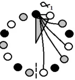
to the opposite region will contribute an edge to the cut. Thus, the top black vertex will

contribute a total of r edges to the cut of region α1. As you can see in Figure 1.10 only

the grey and white vertices clockwise from the top black vertex to the opposite region

will contribute an edge to the cut of region α1.

(28)

We now need to consider the remainingr−1 black vertices. There will be r−₂1 black vertices clockwise from the top black vertex to its opposite region and r−₂1 black

vertices counter-clockwise from the top black vertex to its opposite region. Also, there

will be a combination of r grey and white vertices clockwise from a black vertex to its

opposite region and the remaining r grey and white vertices counter-clockwise from the

same black vertex to its opposite region. Therefore, between each pair of consecutive

black vertices there will be one grey vertex and one white vertex. Thus, each black

vertex clockwise and counter-clockwise from the top black vertex to its opposite region

will have a multiple of two grey and white vertices between the top black vertex and the

black vertex being considered. As you can see in Figure 1.11 there are two black vertices

clockwise and counter-clockwise from the top black vertex to its opposite region. There

is one grey vertex and one white vertex between each black vertex.

Figure 1.11: Remaining r−1 Black Vertices Arrangement ofK5,5,5

Let’s consider the first black vertex clockwise from the top black vertex. The

grey and white vertices clockwise to this black vertex to its opposite region will not

contribute any edges to the cut of region α1. So consider the remainingr grey and white

vertices counter-clockwise. There will be two grey and white vertices between this black

vertex and the top black vertex that also will not contribute any edges to the cut of region

α1. However, the remainingr−2 grey and white vertices will each contribute an edge to

(29)

Figure 1.12: First Clockwise Black Vertex Edge Contribution to α1 ofK5,5,5

Now consider the second black vertex clockwise from the top black vertex.

Sim-ilarly the grey and white vertices clockwise to this black vertex to its opposite region will

not contribute any edges to the cut of region α1. Considering the remaining r grey and

white vertices counter-clockwise, there will be four grey and white vertices between this

black vertex and the top black vertex that will also not contribute any edges to the cut

of region α1. Therefore, the remaining r−4 grey and white vertices will each contribute

an edge to the cut of region α1.

Figure 1.13: Second Clockwise Black Vertex Edge Contribution toα1 of K5,5,5

This pattern will continue until we reach the region opposite the top black

ver-tex. Thus, the total edges contributing to the cut of regionα1 from each r−₂1 black vertex

(30)

[r−2] + [r−4] +...+ [r−2 r−₂1] =

r−1 2

P

n=1

[r−2n]

=

r−1 2

P

n=1 r−2

r−1 2

P

n=1 n

= r r−₂1−2

_r−1 2 (

r−1 2 +1) 2

= r2−2₄r+1

Considering the other r−₂1 black vertices counter-clockwise from the top black

vertex, the same pattern will occur contributing another r2−2₄r+1 edges to the cut of

re-gion α1.

Now we need to consider the edges connecting the grey vertices to the white

vertices that will contribute to the cut of region α1. There will be r−₂1 grey vertices

clockwise from the top black vertex to its opposite region and r+1₂ grey vertices

counter-clockwise from the top black vertex to its opposite region. Let’s consider the grey vertices

clockwise to the top black vertex first. For each grey vertex clockwise to the top black

vertex to the region opposite it there are r−₂1 white vertices clockwise to the grey vertex

being considered that will not contribute an edge to the cut of region α1. However,

there are r+1₂ white vertices counter-clockwise to each of these grey vertices that need

to be considered. So let’s look at the first grey vertex clockwise to the top black vertex.

There is one white vertex between this grey vertex and the top black vertex that will not

contribute an edge to the cut of regionα1. However, the remaining r+1₂ −1 white vertices

(31)

Figure 1.14: First Clockwise Grey Vertex Edge Contribution toα1 of K5,5,5

Now consider the second grey vertex clockwise to the top grey vertex. Note

between consecutive grey vertices there is one white vertex. Also between any two grey

vertices there is a multiple of of white vertices. So considering the second grey vertex

clockwise to the top black vertex, we now have two white vertices between the top black

vertex and the second grey vertex that will not contribute any edges to the cut of region

α1. However, the remaining r+1₂ −2 white vertices counter-clockwise to this grey vertex

will each contribute an edge to the cut of region α1.

Figure 1.15: Second Clockwise Grey Vertex Edge Contribution to α1 of K5,5,5

This pattern will continue until the last grey vertex just before the region

op-posite the top black vertex is reached. Thus, the total edges contributing to the cut of

(32)

[r+1₂ −1] + [r+1₂ −2]+ ... +[r+1₂ −r−1 2 ]

=

r−1 2

P

n=1

_r₊₁

2 −n

= 1₂

"r−1 2

P

n=1 r+

r−1 2 P n=1 1 # −

r−1 2

P

n=1 n

= 1₂r r−₂1+r−₂1−

_r₋₁

2 ( r−1

2 +1) 2

= r2₈−1

Now consider the other r+1₂ grey vertices counter-clockwise from the top black

vertex to the region opposite of it. Note, for each grey vertex counter-clockwise to the top

black vertex to the region opposite it there are now r+1₂ white vertices counter-clockwise

to the grey vertex being considered that will not contribute any edges to the cut of region

α1. However, there are r−₂1 white vertices clockwise to each of these grey vertices that

need to be considered. So let’s look at the first grey vertex counter-clockwise to the top

black vertex. Now there are no white vertices between this grey vertex and the top black

vertex. Thus, all r−₂1 white vertices clockwise to this grey vertex will each contribute an

(33)

Figure 1.16: First Counter-Clockwise Grey Vertex Edge Contribution to α1 of K5,5,5

Also between consecutive grey vertices there is still one white vertex, and

be-tween any two grey vertices there is still a multiple of white vertices. So a pattern

similar to the other grey vertices occurs. Thus, the total edges contributing to the cut of

regionα1from each r+1₂ grey vertex clockwise from the top black vertex will be as follows.

[r−₂1] + [r−₂1 −1] + [r−₂1 −2]+ ... +[r−₂1 − r+1₂ −1

] = r+1 2 P n=1 _r−₁

2 −(n−1)

= 1₂

"r+1 2 P n=1 r− r+1 2 P n=1 1 # − r+1 2 P n=1 n+ r+1 2 P n=1 1

= 1₂

r r+1₂

−r+1 2 − _r₊₁ 2 ( r+1

2 +1) 2

+ r+1₂

= r2₈−1

Now that all possible edges contributing to the cut of regionα1 have been

(34)

cut(α1) = r+ 2

r2₋₂_r₊₁ 4

+ 2

r2₋₁ 8

= 3r2₄+1

Now let’s consider the other regions within the set of one black vertex, one grey

vertex, and one white vertex that will have a similar cut to the regionα1. The cut of the

region immediately clockwise to the white vertex and the cut of the region immediately

clockwise to the grey vertex will be equal to the cut of regionα1 since all the regions are

symmetrical.

Since the cut of all regions for this cyclic arrangement have been evaluated, we

claim the upperbound for the cyclic cutwidth of Kr,r,r forr odd is,

ccw(Kr,r,r)≤ 3r

2₊₁ 4

Also, since the upper bound and the lower bound are the same, we claim the

cyclic cutwidth of Kr,r,r forr odd is,

ccw(Kr,r,r) = 3r

2₊₁ 4

Theorem 7 and Theorem 8 only scratch the surface of cyclic cutwidth of complete

tripartite graphs. In Chapter 2 we explore a new case for the cyclic cutwidth of complete

(35)

Chapter 2

Cyclic Cutwidth of Complete

Tripartite Graph

K

r,r,pr

For

r

Odd

and

p

a Natural Number

In this chapter we are going to explore the cyclic cutwidth of complete tripartite

graph Kr,r,pr, where r is odd and p is a natural number. In order to find the cyclic

cutwidth we will find a lower and upper bound and show that they match. When looking

at both bounds two cases develop, when p is even and whenp is odd.

Theorem 9. For a complete tripartite graph Kr,r,pr where r is odd and p a natural

number, the cyclic cutwidth is,

ccw(Kr,r,pr) =

  

(2p+1)r2₊₁

4 forp odd

(2p+1)r2₊₃

4 forp even

Proof. To show the cyclic cutwidth ofKr,r,pris as stated above we need to show the lower

bound and upper bound are equivalent. Consider the following.

2.1

Lower Bound

By lemma 1, a lower bound of the cyclic cutwidth for any complete tripartite

(36)

Using lemma 1 consider the complete tripartite graphKr,r,pr wherer is odd and

p a natural number. The lower bound is as follows.

ccw(Kr,r,pr) ≥ rr+r(pr₄)+r(pr)

≥ (2p+1)₄ r2

However, (2p+1)₄ r2 is not an integer. There are two cases when rounding up to

the next integer, p being odd andp being even.

2.1.1 Case 1: p is Odd

p is odd. Letp= 2n+ 1 wheren= 1,2,3.... Then,

2p+ 1 = 2(2n+ 1) + 1

= 4n+ 3

≡ 3(mod 4)

(37)

(2p+ 1)r2 ≡ 3r2(mod 4)

≡ 3(2m+ 1)2_{(mod 4)}

≡ 3(4m2+ 4m+ 1)(mod 4)

≡ 3(mod 4)

Thus, (2p+ 1)r2+ 1≡0(mod 4) hence 4|(2p+ 1)r2+ 1. Therefore, to round up to the next integer we would need to add one to the numerator. Thus, when p is odd a

lower bound for the cyclic cutwidth of Kr,r,pr withr odd is,

ccw(Kr,r,pr)≥ (2p+1)r

2₊₁ 4

2.1.2 Case 2: p is Even

p is even. Letp= 2nwhere n= 1,2,3.... Then,

2p+ 1 = 2(2n) + 1

= 4n+ 1

≡ 1(mod 4)

(38)

(2p+ 1)r2 ≡ r2(mod 4)

≡ (2m+ 1)2_{(mod 4)}

≡ 4m2+ 4m+ 1(mod 4)

≡ 1(mod 4)

Thus, (2p+ 1)r2 + 3 ≡ 0(mod 4) hence 4|(2p+ 1)r2 + 3. Therefore, to round up to the next integer we would need to add 3 to the numerator. Thus, whenp is even a

lower bound for the cyclic cutwidth of Kr,r,pr withr odd is,

ccw(Kr,r,pr)≥ (2p+1)r

2₊₃ 4

Therefore, for a complete tripartite graphKr,r,pr whereris odd andpa natural

number, a lower bound of the cyclic cutwidth is,

ccw(Kr,r,pr)≥

  

(2p+1)r2₊₁

4 forp odd

(2p+1)r2₊₃

4 forp even

2.2

Upper Bound

A specific arrangement will be used to come up with an upperbound. Within the

arrangement we are going to look for a region that has the maximum cut. LetV1 consist

of r black vertices, V2 consist of r grey vertices, andV3 consist of prwhite vertices. We

will maker groups of vertices consisting of one black vertex, one grey vertex andpwhite

vertices. Within each cyclic embedding the vertices will be arranged clockwise starting

with a black vertex at the top followed by p₂ white vertices, then a grey vertex followed

by another p₂ white vertices. If p is even then p₂ is an integer andp white vertices will

be evenly distributed between consecutive black and grey vertices. If p is odd then p₂ is

(39)

the black vertex and ₂ white vertices immediately clockwise to the grey vertex. This

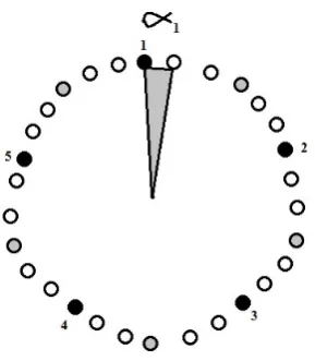
pattern will continue until all (p+ 2)rvertices have been placed. Figure 2.1 is an example

of this arrangement for K3,3,6 and K3,3,9.

Figure 2.1: Vertex Arrangement for Kr,r,pr

This arrangement minimizes the number of regions we need to consider for the

maximum cut. Since each set of black, grey and white vertices is a repeated pattern, the

cuts for each similar region will also be repeated. Thus, we only need to consider the

different regions within one set of black, grey, and white vertices.

As each region is considered for the upper bound of the cyclic cutwidth two cases

develop, whenpis even and whenpis odd. Whenpis even, we need to consider diameters

and how that will affect the maximum cut. When pis odd, there will be no diameters to

consider; however, the white vertices will no longer be grouped evenly between each black

and grey vertex. In either case the non-diameter edges will take the shortest route within

the cyclic embedding to connect two vertices. This will ensure each cut to be minimized

such that not one or more regions are overloaded with edges. So consider the following

two cases.

2.2.1 Case 1: p is Even

Letp be even. Recall when p is even the arrangement will consist of one black

(40)

vertices and then the pattern repeats. With this case we need to consider two different

regions where the maximum cut may lie, the region immediately clockwise to the black

vertex, call it α1, and the region immediately clockwise of the first white vertex, call it

α2. The remaining regions will be similar to either region α1 or region α2 and will be

discussed further after an upperbound of the cyclic cutwidth is found for region α1 and

region α2.

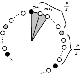
Figure 2.2: Regions α1 and α2

Consider region α1. To get the cut of this region we will look at the vertices

whose edges contribute to the cut. We will look at them in the following order:

diame-ters, the top black vertex connecting to the grey and white vertices, the remaining black

vertices connecting to the grey and white vertices, and the grey vertices connecting to

the white vertices.

Let’s first consider the diameters. In this arrangement for every black vertex

there will be one grey vertex directly across from it within the cyclic embedding. Also

directly across from a white vertex there will always be another white vertex. Since white

vertices cannot connect to white vertices, there will only ber diameters connecting each

black vertex to the one grey vertex directly across from it. Since the diameters cannot

travel straight through the center of the cyclic embedding, we will alternate each

diame-ter clockwise then coundiame-ter-clockwise around the cendiame-ter as shown in Figure 2.3. This will

minimize the number of diameters crossing through each region. Therefore, either r−₂1

diameters or r+1₂ diameters will be contributing to the cut of each region . Since we are

(41)

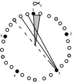
Figure 2.3: Diameters ofK5,5,20

Now let’s consider the edges connecting the top black vertex to the grey and

white vertices that will contribute to the cut of region α1. Since the edge connecting

the top black vertex to the bottom grey vertex directly across from it is included in the

diameters we will consider the grey and white vertices clockwise from the top black vertex

to the bottom grey vertex and the grey and white vertices counter-clockwise from the top

black vertex to the bottom grey vertex. There will be pr₂ white vertices clockwise from

the top black vertex to the bottom grey vertex and pr₂ white vertices counter-clockwise

from the top black vertex to the bottom grey vertex. There will also be r−₂1 grey vertices

clockwise from the top black vertex to the bottom grey vertex and r−₂1 grey vertices

counter-clockwise from the top black vertex to the bottom grey vertex. The grey and

white vertices counter-clockwise from the top black vertex to the bottom grey vertex will

not contribute any edges to the cut of region α1. However, each grey and white vertex

clockwise from the top black vertex to the bottom grey vertex will contribute an edge

to the cut. Thus, the top black vertex will contribute a total of pr₂ +r−₂1 edges to the

cut of region α1. As you can see in Figure 2.4 only the grey and white vertices clockwise

from the top black vertex to the bottom grey vertex will contribute an edge to the cut of

(42)

Figure 2.4: Top Black Vertex Edge Contribution toα1 of K5,5,20

We now need to consider the remainingr−1 black vertices. There will be r−₂1 black vertices clockwise from the top black vertex to the bottom grey vertex and r−₂1 black

vertices counter-clockwise from the top black vertex to the bottom grey vertex. Recall

that each black vertex will be directly across from a grey vertex and will be connected

by a diameter. Since the edges connecting a black vertex to its opposite grey vertex were

already considered with the diameters they will not be counted here. Thus, there will be

pr

2 white vertices clockwise from a black vertex to its opposite grey vertex and

pr

2 white

vertices counter-clockwise from the same black vertex to its opposite grey vertex. As well

there will be r−₂1 grey vertices clockwise from the same black vertex to its opposite grey

vertex and r−₂1 grey vertices counter-clockwise from the same black vertex to its opposite

grey vertex. Therefore, between each pair of consecutive black vertices there will be a set

ofp+ 1 grey and white vertices. Thus, each black vertex clockwise and counter-clockwise

from the top black vertex to the bottom grey vertex will have a multiple ofp+ 1 grey and

white vertices between the top black vertex and the black vertex being considered. As you

can see in Figure 2.5 there are two black vertices clockwise and counter-clockwise from

the top black vertex to the bottom grey vertex. There is a total of five grey and white

vertices between each black vertex, one grey vertex and four white vertices. Consider

the black vertex 3 in Figure 2.5. There are two sets of grey and white vertices between

the top black vertex and black vertex 3, making a total of ten grey and white vertices

(43)

Figure 2.5: Remaining r−1 Black Vertices Arrangement ofK5,5,20

Let’s consider the first black vertex clockwise from the top black vertex. The

grey and white vertices clockwise to this black vertex to the grey vertex directly across

from it will not contribute any edges to the cut of region α1. So consider the remaining

pr

2 +

r−1

2 grey and white vertices counter-clockwise. There will be p+ 1 grey and white

vertices between this black vertex and the top black vertex that also will not contribute

any edges to the cut of region α1. However, the remaining pr₂ + r−₂1 −(p+ 1) grey and

white vertices will each contribute an edge to the cut of region α1. See Figure 2.6 for an

example.

(44)

Now consider the second black vertex clockwise from the top black vertex.

Simi-larly the grey and white vertices clockwise to this black vertex to the grey vertex directly

across from it will not contribute any edges to the cut of region α1. Considering the

remaining pr₂ +r−₂1 grey and white vertices counter-clockwise, there will be 2(p+ 1) grey

and white vertices between this black vertex and the top black vertex that will also not

contribute any edges to the cut of regionα1. Therefore, the remaining pr₂ +r−₂1−2(p+ 1)

grey and white vertices will each contribute an edge to the cut of region α1. See Figure

2.7 for an example.

Figure 2.7: Second Clockwise Black Vertex Edge Contribution toα1 of K5,5,20

This pattern will continue until we reach the last black vertex just before the

bottom grey vertex. Thus, the total edges contributing to the cut of region α1 from each

r−1

(45)

[pr₂ +r−₂1 −(p+ 1)] + [pr₂ + r−₂1−2(p+ 1)] +...+p₂

= (p+1)(r−₂ 2)−1+ (p+1)(₂r−4)−1 +...+ (p+1)(r−₂(r−1))−1

=

r−1 2

P

n=1

(p+1)(r−2n)−1 2

= p+1₂

"r−1 2

P

n=1 r−2

r−1 2 P n=1 n # −

r−1 2

P

n=1 1 2

= p+1₂

r−1 2

r−2

(r−1 2 )(

r−1 2 +1) 2

−1₂ r−₂1

= (p+1)(₈r−1)2 −r−₄1

Considering the other r−₂1 black vertices counter-clockwise from the top black

vertex, the same pattern will occur contributing another (p+1)(₈r−1)2 − r−₄1 edges to the cut of regionα1.

Now we need to consider the edges connecting the grey vertices to the white

vertices that will contribute to the cut of region α1. First consider the bottom grey

vertex. The white vertices clockwise from the bottom grey vertex to the top black vertex

will contibute no edges to the cut of region α1 as shown in Figure 2.8. Similarly the

white vertices counter-clockwise from the bottom grey vertex to the top black vertex will

contribute no edges to the cut of regionα1. Thus, we only need to consider the remainig

(46)

Figure 2.8: Botttom Grey Vertex Edge Contribution toα1 of K5,5,20

There will be r−₂1 grey vertices clockwise from the top black vertex to the bottom

grey vertex and r−₂1 grey vertices counter-clockwise from the top black vertex to the

bottom grey vertex. Recall that each grey vertex will be directly across from a black

vertex. Thus, there will be pr₂ white vertices clockwise to a grey vertex to its opposite

black vertex and pr₂ white vertices counter-clockwise to the same grey vertex to its opposite

black vertex. Therefore, between each pair of consecutive grey vertices there will be a set

ofpwhite vertices and between each pair of consecutive grey and black vertices there will

be a set of p₂ white vertices. Thus, each grey vertex clockwise and counter-clockwise from

the top black vertex to the bottom grey vertex will have a multiple of p₂ white vertices

between the top black vertex and the grey vertex being considered. As you can see in

Figure 2.9 there are two grey vertices clockwise and counter-clockwise from the top black

vertex to the bottom grey vertex. Also there are two white vertices between consecutive

grey and black vertices and four white vertices between consecutive grey vertices. For

example, grey vertex 2 has three sets of two white vertices between the top black vertex

(47)

Figure 2.9: Grey vertex Placement ofK5,5,20

Let’s consider the first grey vertex clockwise from the top black vertex. The

white vertices clockwise of this grey vertex to the black vertex directly across from it will

not contribute any edges to the cut of region α1. So consider the remaining pr₂ white

vertices counter-clockwise. There will be p₂ white vertices between this grey vertex and

the top black vertex that also will not contribute any edges to the cut of region α1.

However, the remaining pr₂ −p₂ white vertices will each contribute an edge to the cut of region α1. See Figure 2.10 for an example.

Figure 2.10: First Clockwise Grey Vertex Edge Contribution toα1 of K5,5,20

(48)

white vertices clockwise to this grey vertex to the black vertex directly across from it will

not contribute any edges to the cut of region α1. So consider the remaining pr₂ white

vertices counter-clockwise. There will be 3 p₂

white vertices between this grey vertex

and the top black vertex that also will not contribute any edges to the cut of region α1.

However, the remaining pr₂ −3 p₂

white vertices will each contribute an edge to the cut

of region α1. See Figure 2.11 for an example.

Figure 2.11: Second Clockwise Grey Vertex Edge Contribution to α1 ofK5,5,20

This pattern will continue until we reach the last grey vertex just before the

bottom grey vertex. Thus, the total edges contributing to the cut of region α1 from each

r−1

(49)

[pr₂ −p₂] + [pr₂ −3₂p] + [pr₂ −5₂p] +...+ 0

= p(r−₂1)+ p(r−₂3) +...+p(r−r₂ )

=

r+1 2

P

n=1

p[r−(2n−1)] 2

= p₂

"r+1 2

P

n=1 r−2

r+1 2 P n=1 n+ r+1 2 P n=1 1 #

= p₂

r r+1₂ −2

(r+1 2 )(

r+1 2 +1) 2

+ r+1₂

= p(r+1)(₈r−1)

Considering the other r−₂1 grey vertices counter-clockwise from the top black

vertex the same pattern will occur contributing another p(r+1)(₈r−1) edges to the cut of

region α1.

con-sidered, the total edges contributing to the cut are as follows.

cut(α1) = r(p+1)

−1

2 +

r+1 2 + 2

h₍_p₊₁₎₍_r−₁₎2

8 −

r−1 4

i

+ 2hp(r+1)(₈r−1)i

= (2p+1)₄r2+3

Now let’s consider the other cuts within the set of one black vertex, one grey

vertex, and p white vertices that will have a similar cut to the region α1. The cut of

the region immediately counter-clockwise to the black vertex will be less than or equal

(50)

will contribute an equivalent number of edges to the cut. The edges from diameters will

contribute the same number of edges or one edge less than the region adjacent to it.

Since the number of black vertices is equivalent to the number of grey vertices and the

arrangement of the cyclic embedding is symmetrical, the region immediately clockwise

and counter-clockwise to the grey vertex will also be less than or equal to the cut of region

α1 for the same reasons.

Now that an upper bound has been found for the region α1 and the regions

similar to it, we now need to consider the remaining regions. So consider regionα2.

Figure 2.12: Regions α1 and α2

To get the cut of this region we will look at the vertices whose edges contribute

to the cut. We will look at them in the following order: the first set of white vertices

clockwise to the top black vertex connecting to the black and grey vertices, the other sets

of white vertices connecting to the black and grey vertices, the diagonals connecting each

black vertex to its opposite grey vertex, and the other black vertices connecting to the

grey vertices.

Let’s consider the first set of white vertices clockwise from the top black vertex.

There are p₂ white vertices in this set. Also there is a combination of r black and grey

vertices clockwise from this set of white vertices to the set of white vertices opposite of

them and the remainingrblack and grey vertices counter-clockwise from this set of white

vertices to the set of white vertices opposite of them. As shown in Figure 2.13 there are

(51)

vertices clockwise from the top black vertex to the set of white vertices opposite of them.

Figure 2.13: Region α2 ofK3,3,24

Consider the first white vertex clockwise from the top black vertex. The

com-bination of r black and grey vertices counter-clockwise to this white vertex to the white

vertex opposite of it, will not contribute any edges to the cut of region α2. However, the

remaining r black and grey vertices clockwise to this white vertex to the white vertex

opposite it, will each contribute an edge to the cut of region α2.

Figure 2.14: First Clockwise White Vertex Edge Contribution to α2 ofK3,3,24

(52)

black and grey vertices clockwise to this white vertex to the white vertex opposite of it

will not contribute any edges to the cut of region α2. However,r black and grey vertices

counter-clockwise to the white vertex to the white vertex opposite it will each contribute

an edge to the cut of region α2. This pattern will continue for each white vertex in the

first set of white vertices clockwise to the top black vertex. Thus, this set of white vertices

will contribute a total of r p₂ edges to the cut of the regionα2.

Figure 2.15: Second and Third Clockwise White Vertex Edge Contribution toα2ofK3,3,24

Now we need to consider the remaining white vertices. We are first going to

look at each set of white vertices clockwise from the first set of white vertices we just

considered and then look at the set of white vertices counter-clockwise to the same set.

For each white vertex in the first set of white vertices clockwise to the set of white vertices

of region α2, there is a combination of r black and grey vertices clockwise and

counter-clockwise to this set of white vertices. The r black and grey vertices clockwise to the

set of white vertices will contribute no edges to the cut of the region α2. So consider

the remaining r black and grey vertices counter-clockwise to the set of white vertices

being considered. There is now one grey vertex between the first and second set of white

vertices that will not contribute an edge to the cut of the region α2. Thus, there will be

r−1 edges contributing to the cut of the region α2 from each white vertex in this set,

(53)

Figure 2.16: Second Set of Clockwise White Vertex Edge Contribution to α2 ofK3,3,24

This same pattern happens for each set of white vertices clockwise from the first

set. However, for each set you move clockwise, there is an additional grey or black vertex

between the first set of white vertices and the set of white vertices being considered. For

example, for the third set of white vertices clockwise from the top black vertex there will

be two grey and black vertices between the first and third set of white vertices resulting

inr−2 edges contributing to the cut of the region ofα2. This makes a total of (r−2) p₂

edges contributing to the cut of the regionα2from the third set of white vertices clockwise

from the top black vertex. So the fourth set of white vertices will contribute a total of

(r−3) p₂edges to the cut of the regionα2. Continuing this pattern for each set of white

vertices clockwise to the set of white vertices containing α2 we will have the following

(54)

[p₂(r−1)] + [p₂(r−2)] + [₂p(r−3)] +... + [p₂(r−r)]

=

r

P

n=1

p

2(r−n)

= p₂

_r P

n=1 r−

r

P

n=1 n

= p₂

h

r(r)−r(r₂+1)i

= p(r2₄−r)

Considering the other sets of white vertices counter-clockwise from the top black

vertex the same pattern will occur contributing another p(r2₄−r) edges to the cut of region

α2.

Now let’s consider the diameters. Recall in this arrangement for every black

ver-tex there will be a grey verver-tex directly across from it within the cyclic embedding. Also

directly across from a white vertex there will always be another white vertex. Since white

vertices cannot connect to white vertices there will only be r diameters connecting each

black vertex to the one grey vertex directly across from it. Since the diameters cannot

travel straight through the center of the cyclic embedding we will alternate each diameter

clockwise then counter-clockwise around the center as shown in Figure 2.17. This will

minimize the number of diameters crossing through each region. Therefore, either r−₂1

diameters or r+1₂ diameters will be contributing to the cut of each region . Since we are

(55)

Figure 2.17: Diameters Contributing to The Cut of Regionα2 of K3,3,24

The last set of edges that need to be considered are the non-diameter edges

connecting black vertices to the grey vertices. So for each black vertex there are r−₂1

grey vertices clockwise and counter-clockwise to the black vertex being considered to

the grey vertex directly across from it. The top black vertex will contribute r−₂1 edges

to the cut of region α2 by connecting to each r−₂1 grey vertices clockwise to the top

black vertex. Now consider the black vertices clockwise from the top black vertex to the

bottom grey vertex. The edges connecting to the grey vertices clockwise from each black

vertex will not contribute any edges to the cut of regionα2. So consider the grey vertices

counterclockwise to each black vertex. The top black vertex and the black vertex being

considered will have a multiple of grey vertices between them that will not contribute an

edge to the cut of region α2. This number of grey vertices will increase by an increment

of one for each black vertex that is farther from the top black vertex. Thus, the first

black vertex clockwise from the top black vertex will contribute r−₂1−1 edges, the second black vertex clockwise from the top black vertex will contribute r−₂1 −2 edges, and the third black vertex clockwise from the top black vertex will contribute r−₂1−3 edges. This pattern will continue until the last black vertex clockwise from the top black vertex just

before the bottom grey vertex is reached. Thus, the black vertices clockwise from the top

(56)

[r−₂1 −1] + [r−₂1−2] + [r−₂1 −3] +... + [r−₂1 −r−1 2 ]

=

r−1 2

P

n=1

r−1 2 −n

= 1₂

"r−1 2

P

n=1 r−