OPTIMIZATION OF MACHINING
PARAMETERS IN TURNING PROCESS
USING GENETIC ALGORITHM AND
PARTICLE SWARM OPTIMIZATION
WITH EXPERIMENTAL
VERIFICATION
H.GANESAN
Department of Mechanical Engineering, RVS College of Engineering & Technology
Coimbatore, Tamilnadu, India
G.MOHANKUMAR, K.GANESAN, K.RAMESH KUMAR
Department of Mechanical Engineering, Park College of Engineering & Technology
Coimbatore, Tamilnadu, India
Department of Mechanical Engineering, PSG College of Technology Coimbatore, Tamilnadu, India
Department of Mechanical Engineering, Amritha School of Engineering & Technology
Coimbatore, Tamilnadu, India
ABSTRACT
Optimization of cutting parameters is one of the most important elements in any process planning of metal parts. Economy of machining operation plays a key role in competitiveness in the market. All CNC machines produce finished components from cylindrical bar. Finished profiles consist of straight turning, facing, taper and circular machining. Finished profile from a cylindrical bar is done in two stages, rough machining and finish machining. Numbers of passes are required for rough machining and single pass is required for the finished pass. The machining parameters in multipass turning are depth of cut, cutting speed and feed. The machining performance is measured by the minimum production time.
In this paper the optimal machining parameters for continuous profile machining are determined with respect to the minimum production time, subject to a set of practical constraints, cutting force, power and dimensional accuracy and surface finish. Due to complexity of this machining optimization problem, a genetic algorithm (GA) and Particle Swarm Optimization (PSO) are applied to resolve the problem and the results obtained from GA and PSO are compared.
1. INTRODUCTION
It has long been recognized that conditions during cutting, such as feed rate, cutting speed and depth of cut, should be selected to optimize the economics of machining operations as assessed by productivity, total manufacturing cost per component or some other suitable criterion. Hinduja et al [1]described a procedure to calculate the optimum cutting conditions for turning operations with minimum cost or maximum production rate as the objective function. For a given combination of tool and work material, the search for the optimum was confined to a feed rate versus depth-of-cut plane defined by the chip-breaking constraint. Some of the other constraints considered include power available, work holding, surface finish and dimensional accuracy.
Agapiou [2] formulated single-pass and multi-pass machining operations. Production cost and total time were taken as objectives and a weighting factor was assigned to prioritize the two objectives in the objective function. The author optimized the number of passes, depth of cut, cutting speed and feed rate in his model, through a multi-stage solution process called dynamic programming. Several physical constraints were considered and applied in this model. In his solution methodology, every cutting pass is independent of the previous pass, hence the optimality for each pass is not reached simultaneously. Agapiou used a dynamic programming model similar to that of Iwta[3] for determining the optimum value of an objective function (weighted sum of production cost and time) and Ruy Mesquita [4] used the Hook–Jeeves search method for finding the optimum operating parameters. Shin and Joo [5] have presented a model for multipass turning .In the above research, only the straight turning process, i.e. cutting a component in the longitudinal direction to produce a constant part diameter, was discussed. The finished component from CNC, in an FMS environment contains a continuous profile. The continuous profile consists of straight turning, facing, taper turning, convex and concave circular arcs. Yellowley et. al [6]. have shown that for both turning and milling operations the optimal subdivision of depth of cut may be determined without knowledge of the relevant tool life equation. Calculation of machining parameters in turning operation using machining theory was carried out by Menget al.[7]. The objective criteria used in this work is minimum cost. Prased et. al.[8] have used the combination of geometric and linear programming techniques for solving multi-pass turning optimization problem as part of a PC-based generative Computer Aided Process Planning (CAPP) system. Onwubolu et al. [9] have used a genetic algorithm for optimizing multipass turning operations. Multipass turning optimization with optimal subdivision of depth of cut was developed by Gupta et al. [10]
Savaranan et. al [11]. have used a GA, SA, Nelder–Meadsimplex and a Boundary search procedure for optimizing a CNC turning process, but the work was limited to straight turning only. Contour profile was not considered in this work. The computation time of the algorithms was also observed and MOPSO has been found to have a vastly superior execution time compared to the other algorithms. This is attributed to the adaptive grid used by MOPSO which has lower computational cost [12] than the crowding distance used by NSGA-II combined with the non dominated sorting as suggested by Goldberg [13]. The proposed algorithm extends PSO in solving multi objective optimization problems by incorporating the mechanism of crowding distance computation in the global best selection and the deletion method of the external archive of non dominated solutions whenever the archive is full. The crowding distance mechanism together with a mutation operator maintains the diversity of non dominated solutions in the external archive.
.Most of the researchers in the area of machining have usedvarious techniques for finding the optimal machining parameters for single- and multipass turning operations..Traditional techniques are not efficient when the practical search space is too large. Considering the drawbacks of traditional optimization techniques,
The following table shows the some of the objective functions and constraints considered
Sl.
No. Area of Investigation
Objective Functions Considered
Constraint Considered
Year of Publications
1
Optimizing cutting parameters in process planning of prismatic parts by using genetic algorithms
a) Minimum Production time
b) Minimum Production cost
a) Power b) Surface finish
2
Machining Parameters Optimization for turning Cylindrical stock into a continuous finished profile using GA & SA
a) Minimize the cost
a) Cutting speed b) Cutting force c) power
d) Chip tool inter face
e)Dimensional Accuracy f) S f Fi i h
(2003)
3 Optimization of cutting conditions during continuous finished profile machining using non traditional techniques
a) Minimum Production cost
a) Tool life b) Cutting force c) Power
d) Stable cutting region
e)Dimensional accuracy
( 2005)
4 Genetic algorithm based multi objective optimization of cutting parameters in turning processes
a) Production rate b) Tool rate
a) Depth of cut b) Feed rate c) Cutting speed d) Cutting force e) Cutting power f) Surface roughness
(2006)
This paper attempts to determine the optimal machining parameters for machining of a continuous finished profile from bar stock to minimize the production time using Genetic Algorithm (GA) and Particle Swarm Optimization (PSO) and the results are compared.
.
2. PROBLEM FORMULATION
Turning isa metal cutting process in which the cutting tool enters and leaves the work piece. In CNC machine tools, the finished component is obtained by a number of rough passes and finished pass. The roughing operation is carried out to machine the part to a size that is slightly larger than the desired size, in preparation for the finishing cut. The finishing cut is called single-pass contour machining, and is machined along the profile contour. In this paper, a turning centre with control system is used. Roughing stages and a finished stage are considered to machine the component from the bar stock. The first roughing stage consists of (n-1) passes where n is the total number of roughing passes, and the last pass of roughing removes the material along the profile contour. In the finish stage material (amount of finish allowance) is removed along the contour of the profile. The machining time criteria are used in this work for finding the performance of the machining operations under practical constraints. The length of cutting path is calculated for each pass in the roughing and finishing stages. Then the cutting time for each pass is calculated for these stages. The objective of this model is to minimize the cutting time.
2.1 Model for Machining Performance:
The objective is the minimum operation time, to measured as the entire time required to carry out to finish the work piece, Eq. (1)
tp = Tm+te(Tm/tl)+[Ti] = (Lj+3/f*n)+te((Lj+3/f*n)/f*d*n)+[Ti] (1) where,
tp = Unit time per work piece (min)
Tm = Cutting/(machining time) time
te = Time required to exchange a tool(min)
tl = Tool life(min)
Ti = Machine idle time
f = feed n = speed d = depth of cut
2.2 Machining Constraints
The practical constraints imposed during the roughing and finishing operations as described by Chen and Su [14] are given below.
2.2.1 Parameter bounds
Bounds on cutting speed in Eq. (2)
VrL ≤ Vr ≤ VrU (2)
where VrL and VrU are the lower and upper bounds of cutting speed in roughing, respectively.
Bounds on feed in Eq. (3)
frL < fr < frU (3)
where frL and frU are the lower and upper bounds of feed in roughing, respectively.
Bounds on depth of cut in Eq.(4)
drL < dr < drU (4)
where drL and drU are the lower and upper bounds of depth of cut respectively.
2.2.2 Cutting force
The expression for the cutting force constraint is given by Eq. (5)
Fr =kf fr FU (5)
where Fr is the cutting force during rough machining, kf, and v are the constants pertaining to a specific tool-work piece combination, and FU is the maximum allowable cutting force (kgf).
2.2.3 Power Constraint
The power constraint is given by Eq. (6)
Pr = ≤ PU (6)
where Pr is the cutting power during rough machining (kW), η is the power efficiency, and PU is the maximum
allowable cutting power (kW).
2.2.4 Dimensional Accuracy Constraint
The regression relation for calculating the dimensional accuracy is given by Eq. (7)
δ =100.66.f 0.9709 d0.4905 V-0.2848 (7)
where δ is the dimensional accuracy, f is the feed rate per revolution, d is the depth of cut, and V is the cutting speed.
2.2.5 Surface Finish Constraint
(8)
where r is the nose radius of cutting tool (mm), Rmax is maximum allowable surface roughness (µm) and fs is the feed.
3. SOLUTION METHODOLOGY
Genetic algorithms (GA) and Particle Swarm Optimization (PSO) are best population search based technique.
3.1 Genetic Algorithm (GA):
GA are different from traditional optimizations in the following ways.
1. GA goes through solution space starting from a group of points and not from a single point. 2. GA search from a population of points and not a single point.
3. GA use information of a fitness function, not derivatives or other auxiliary knowledge. 4. GA use probabilistic transitions rules, not deterministic rules.
5. It is very likely that the expected GA solution will be a global solution.
The cutting conditions are encoded as genes by binary encoding to apply GA in optimization of machining parameters. A set of genes is combined together to form chromosomes, used to perform the basic mechanisms in GA, such as crossover and mutation. GA optimization methodology is based on machining performance predictions models developed from a comprehensive system of theoretical analysis, experimental database and numerical methods. The GA parameters along with relevant objective functions and set of machining performance constraints are imposed on GA optimization methodology to provide optimum cutting conditions.
3.1.1 Genetic Algorithm Methodology
Genetic algorithms are computerized search and optimization algorithms based on the mechanics of natural genetics and natural selection. Optimization can be done by the generation of the population.
3.1.2 Steps in the Genetic Algorithm Optimization
1. Choose a coding to represent problem parameters, a selection operator, a crossover operator, and a mutation operator. Choose population size n, crossover probability pc, and mutation probability pm. Initialize a random population of strings of size l. Choose a maximum allowable generation number tmax. Set t = 0.
2. Evaluate each string in the population.
3. If t tmax or other termination criteria are satisfied, terminate. 4. Perform reproduction on the population.
5. Perform crossover on pair of strings with probability pc. 6. Perform mutation on strings with probability pm.
7. Evaluate strings in the new population. Set * = t + 1 and go to Step 3.
3.1.3 Genetic Algorithm Parameters
Population size: 32 Length of Chromosome: 6 Selection operator: Rank order
Crossover operator: Single point operator Crossover probability: 0.75
Mutation probability: 0.1 Fitness parameter: Operation time
3.1.4 Implementation of GA with Numerical Illustration
are represented as substrings in the chromosome. The strings (000000 0000000 000000) and (111111 111111 111111) represent the lower and upper limits of speed, feed and depth of cut.
3.1.5 Initialization
During initialization, a solution space of a “population size” solution string is generated randomly between the limits of the speed, feed and depth of cut. In this work the solution space size (population size) is considered as 18 as shown in Table 1. Columns 1, Column 2 and 3 show the initial random binary population. Column 4 shows the objective function output (Optimized output). Column 5 denotes the Rank value. Here the binary format population can be decoded by using the below formula.
xi = xi(L) + (decoded decimal value)
Where xi is the decoded speed or feed or depth of cut, x(L) i is the lower limit of speed or feed or depth of cut,
x(U) i is the upper limit of speed or feed or depth of cut, and n is the substring length (= 6).
3.1.6 Evaluation
In a GA, a fitness function value is computed for each string in the population, and the objective is to find a string with the maximum fitness function value. It is often necessary to map the underlying natural objective function to a fitness function form through one or more mappings. Since, we use a minimization objective function, the following transformation is used
f(x) =
Where g(x) is the objective function (Operation time) and f(x) is the fitness function. In the minimization problem the string which has the higher fitness value will be the best string.
3.1.7 Selection and Reproduction
Reproduction selects good strings in a population and forms a mating pool. The reproduction operator is also called a selection operator. In this work rank order selection is used. In Table 1 Column 4 shows the output generated using this method. A lower ranked string will have a lower fitness value or a higher objective function and vice versa.
The higher cumulative probability value in the range is chosen as one of the parents. In Table 1 for the first string the generated random number is 0.237122. The string number(rank) 1, which has a cumulative probability of 0.2485000, is selected as the parent, and this process is repeated for the entire population.
3.1.8 Crossover
Crossover is a mechanism for diversification. The strings to be crossed and the crossing points are selected randomly and crossover is done with a crossover probability. A single-point crossover is used in this work. The crossover probability is 0.75. The concept of crossover is explained below.
Before crossover: 1.110010 – 00 | 0111 2.110100 – 01 | 0010
After crossover: 1&2→9 means crossover takes place between 1st and 2nd string at (9 + 1)th cross site and after the (9 + 1)th bit all the information is exchanged between strings. The cross site number starts from zero. Hence cross site number 9 represents the 10th site.
1.110010 – 01 | 0111 2.110100 – 00 | 0010
3.1.9 Mutation
Mutation is a random modification of a randomly selected string. Mutation is done with a mutation probability of 0.1.
Before mutation: 1. 11001001_0_111
After mutation: 1→9 means that mutation takes place at the 1st string at the 9th site. The mutation will invert from 0 to 1 or 1 to 0 at the particular site.
The output after the first iteration is given in Table 2. The best string in the list is the chromosome rank 1 which has minimum unit production cost. This completes one iteration of the GA and the best value is stored. All the strings available at the end of first iteration will be treated as parents for the second iteration. This procedure is repeated for the number of iterations as given by the user.
In this example,
x i (L)= 50 for speed x i (U) = 3500 for speed x i (L)= 0.01for feed x i(U) = 0.4 for feed x i (L)=0.3 for depth of cut x i (U) = 1.5 for depth of cut
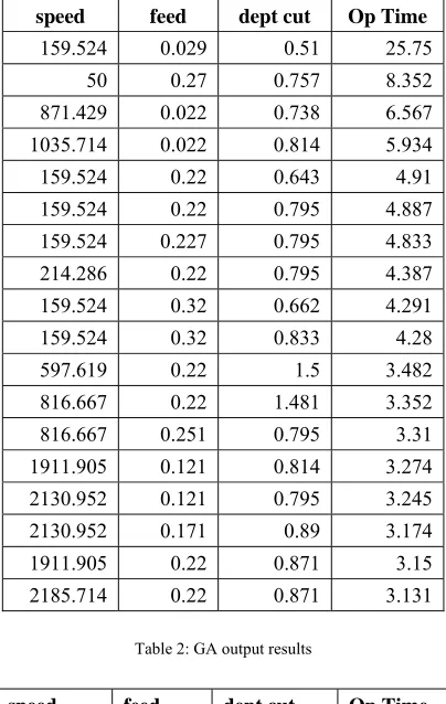
Table 1: The output after the first iteration
speed feed dept cut Op Time
159.524 0.029 0.51 25.75
50 0.27 0.757 8.352 871.429 0.022 0.738 6.567 1035.714 0.022 0.814 5.934 159.524 0.22 0.643 4.91 159.524 0.22 0.795 4.887 159.524 0.227 0.795 4.833 214.286 0.22 0.795 4.387 159.524 0.32 0.662 4.291 159.524 0.32 0.833 4.28
597.619 0.22 1.5 3.482
816.667 0.22 1.481 3.352 816.667 0.251 0.795 3.31 1911.905 0.121 0.814 3.274 2130.952 0.121 0.795 3.245
2130.952 0.171 0.89 3.174
1911.905 0.22 0.871 3.15 2185.714 0.22 0.871 3.131
Table 2: GA output results
speed feed dept cut Op Time 2185.714 0.22 0.871 3.131
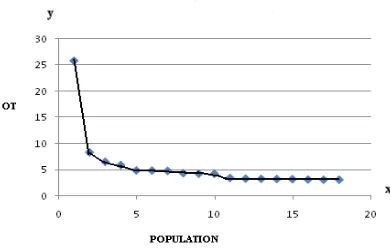
Figure 1 Operation time Vs Population
3.2 PARTICLE SWARM OPTIMIZATION (PSO)
In this proposed algorithm we are using single-objective PSO to optimization problems. Here the mechanism of crowding distance computation is used into the algorithm of PSO specifically on global best selection. The crowding distance mechanism together with a mutation operator maintains the diversity of solutions in the external archive. This also has a constraint handling mechanism for solving constrained optimization problems.
3.2.1 PSO Algorithm
1. For i = 1 to M (M is the population size) a. Initialize P[i] randomly (P is the population of particles)
b. Initialize V[i] = 0 (V is the speed of each particle) c. Evaluate P[i]
d. Initialize the personal best of each particle PBESTS[i] = P[i]
e. GBEST = Best particle found in P[i]
2. End For
3. Initialize the iteration counter t = 0 4. Store the vectors found in P into A
(A is the external archive that stores solutions found in P) 5. Repeat
a. Compute the crowding distance values of each solution in the archive A
b. Sort the solutions in A in descending crowding distance values c. For i = 1 to M
i. Randomly select the global best guide for P[i] from a specified top portion (e.g. top 10%) of the sorted archive A and store its position to GBEST.
ii. Compute the new velocity:
V[i] = W x V[i] + R1 x (PBESTS[i] – P[i]) + R2 x (A[GBEST] – P[i]) (W is the inertia weight equal to 0.4)
(R1 and R2 are random numbers in the range [0..1])
(PBESTS[i] is the best position that the particle i have reached) (A[GBEST] is the global best guide for each solution)
iii. Calculate the new position of P[i]:
P[i] = P[i] + V[i]
v. If (t < (MAXT * PMUT), then perform mutation on P[i]. (MAXT is the maximum number of iterations) (PMUT is the probability of mutation)
vi. Evaluate P[i]
d. End For
e. Insert all new solution in P into A if they are not dominated by any of the stored solutions. All dominated solutions in the archive by the new solution are removed from the archive. If the archive is full, the solution to be replaced is determined by the following steps:
i. Compute the crowding distance values of each solution in the archive A
ii. Sort the solutions in A in descending crowding distance values iii. Randomly select a particle from a specified bottom portion (e.g. lower 10%) which 258 comprise the most crowded particles in the archive then replace it with the new solution
f. Update best solution of each particle in P. If the current PBESTS dominates the position in memory, the particles position is updated using PBESTS[i] = P[i]
g. Increment iteration counter t
6. Until maximum number of iterations is reached
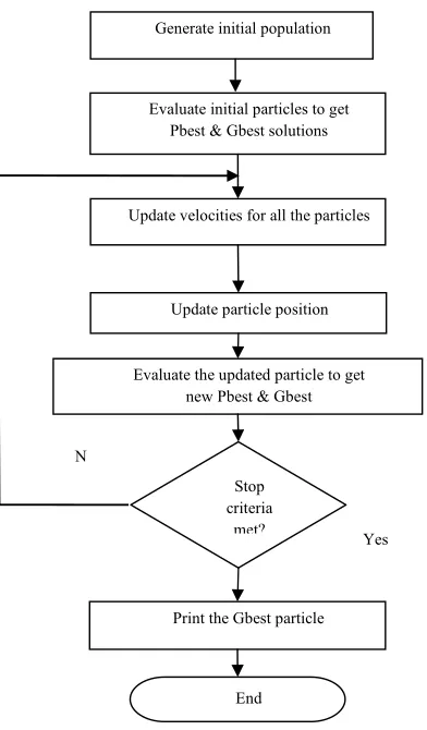
Figure 2: The algorithm for Particle Swarm Optimization
3.2.2 Crowding Distance Computation
Evaluate initial particles to get Pbest & Gbest solutions
Update velocities for all the particles
Update particle position
Evaluate the updated particle to get new Pbest & Gbest
Print the Gbest particle Stop criteria
met?
End Generate initial population
N
The crowding distance value of a solution provides an estimate of the density of solutions surrounding that solution. Crowding distance is calculated by first sorting the set of solutions in ascending objective function values. The crowding distance value of a particular solution is the average distance of its two neighboring solutions. The boundary solutions which have the lowest and highest objective function values are given an infinite crowding distance values so that they are always selected. This process is done for each objective function. The final crowding distance value of a solution is computed by adding the entire individual crowding distance values in each objective function. The pseudo code of crowding distance computation is shown below.
1. Get the number of solutions in the external repository a. n = | S |
2. Initialize distance
a. FOR i=0 TO MAX b. S[i].distance = 0
3. Compute the crowding distance of each solution a. For each objective m
b. Sort using each objective value S = sort(S, m) c. For i=1 to (n-1)
d. S[i].distance = S[i].distance + (S[i+1].m – S[i-1].m)
e. Set the maximum distance to the boundary points so that they are always selected S[0].distance = S[n].distance = maximum distance
3.2.3 Global Best Selection
The selection of the global best guide of the particle swarm is a crucial step in a PSO algorithm. It affects both the convergence capability of the algorithm as well as maintaining a good spread of solutions. we want to ensure that the particles in the population move towards the sparse regions of the search space. In PSO-CD, the global best guide of the particles is selected from among those solutions with the highest crowding distance values. Selecting different guides for each particle in a specified top part of the sorted repository based on a decreasing crowding distance allows the particles in the primary population to move towards those solutions in the external repository which are in the least crowded area in the objective space. Also, whenever the archive is full, crowding distance is again used in selecting which solution to replace in the archive. This promotes diversity among the stored solutions in the archive since those solutions which are in the most crowded areas are most likely to be replaced by a new solution.
3.2.4 Mutation
The mutation operator of PSO was adapted because of the exploratory capability it could give to the algorithm by initially performing mutation on the entire population then rapidly decreasing its coverage over time. This is helpful in terms of preventing premature convergence due to existing local Pareto fronts in some optimization problems.
3.2.5 Constraint Handling
In order to handle constrained optimization problem PSO-CD adapted the constraint handling mechanism used by NSGA-II due to its simplicity in using feasibility and the solutions when comparing final output. A solution i is said to constrained-dominate a solution j if any of the following conditions is true:
1. Solution i is feasible and solution j is not.
2. Both solutions i and j are infeasible, but solution i has a smaller overall constraint violation. 3. Both solutions i and j are feasible and solution i dominates solutions j.
3.2.6 The Time Complexity of PSO-CD
The computational complexity of the algorithm is dominated by the objective function Operation time and Unit of Cost in the archive. If there are M objective functions and N number of solutions (particles) in the population, then the objective function computation has O(MN) computational complexity. The costly part of crowding distance computation is sorting the solutions in each objective function. If there are K solutions in the archive, sorting the solutions in the archive has O(M K log K) computational complexity.
Table 3 PSO Output
Generation No.
Speed Feed Depth of Cut OT
10 3500.000000 0.367393 0.010000 0.000180
4. TEST EXAMPLE
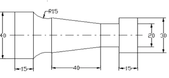
For testing the proposed methodology, the component shown in Fig.3 is considered. The component is to be machined with optimal speed and feed using an SUPER JOBBER LM CNC turning centre in the industry. The work piece material used is EN 8 and the tool material is a carbide tip. The proposed model is run on an FANUC OI TD computer using the C++ language. Tables and graphs summaries the computational results. Number of roughing cuts - 11
Depth of cut for finishing - 0.3 mm
Figure 3. Test Component
5. RESULTS AND DISCUSSION
5.1 Results of Genetic Algorithm
The results obtained from GA and PSO are discussed below. Table 1 shows the optimal cutting parameters such as speed, feed and depth of cut obtained from GA for the minimum Operation time of 3.131 min. Figure 2 shows the fitness obtained in each iteration of the GA. The graph shows that the GA produces smooth fitness at the initial iteration and varying fitness in the subsequent iterations. Using C++ language the optimal solution can be obtained.
Table 3 shows the optimum cutting conditions obtained from PSO for the profile given in Fig. 3 and shows that in the initial stages of the iterations, PSO produces minimum fitness and at the end of the iterations, it gives better results by using C++ language the optimal solution can be obtained.
.
6. CONCLUSION
All types of CNC machines have been used to produce continuous finished profiles. A continuous finished profile has many types of operations such as facing, taper turning and circular turning. To model the machining process, several important operational constraints have been considered. These constraints were taken to account in order to make the model more realistic. A model of the process has been formulated with non-traditional algorithms; GA and PSO have been employed to find the optimal machining parameters for the continuous profile. PSO produces better results. Using this technique machining time can be further minimized.
References
[1] Hinduja S, Petty D J, Tester M, Barrow G 1985 Calculation of optimum cutting conditions for turning operations. Proc. Inst. Mech.
Eng. 199(B2): pp.81–92
[2] Agapiou, “The optimization of machining operations based on a combined criterion, Part-1: the use of combined objectives in single pass operations”, ASME Journal of Engineering for Industry, 114, pp. 500–507, 1992.
[3] K. Iwata et al., “A probabilistic approach to the determination of the optimum cutting conditions”, ASME Journal of Engineering for Industry, 94, pp. 1099–1107, 1972.
[4] Ruy Mesquita et al., “Computer aided selection of optimum machining parameters in multi pass turning”, International Journal of
Advanced Manufacturing technology, 10, pp. 19–26, 1995.
[5] Y. C. Shin, Y. S. Joo, "Optimization of machining conditions with practical constraints", Int. J. Prod. Res., vol. 30, no. 12, pp. 2907– 2919, 1992.
[6] Yellowley et al., “The optimal subdivision of cut in multi passes machining operation”, International Journal of Material Processing Technology, 27, pp. 1572–1578, 1992.
[7] Q. Meng et al., “Calculation of optimum cutting condition for turning operation using a machining theory”, International Journal of Machine Tool and Manufacture, 40,pp. 1709–1733, 2000.
[8] V. S. R. K. Prasad et al., “Optimal selection of process parameters for turning operations in a CAPP system”, International Journal of Production Research, 35, pp.1495–1522, 1997.
[9] G. C. Onwubolu et al., “Multi-pass turning operations optimization based on genetic algorithms”, Proceedings of Institution of
Mechanical Engineers, 215, pp. 117–124, 2001.
[10] R. Gupta et al., “Determination of optimal subdivision of depth of cut in multi-pass turning with constraints”, International Journal of Production Research, 33(9), pp.2555–2565, 1995.
[11] R. Saravanan et.al., “Comparative analysis of conventional and non-conventional optimizations techniques for CNC turning process”, International Journal of Advanced Manufacturing Technology, 17, pp. 471–476, 2001.
[12] Goldberg, D., Genetic Algorithms in Search, Optimization and Machine Learning. Reading, MA: Addison-Wesley, 1989.
[13] Knowles, J. and Corne, D. Approximating the non dominated front using the Pareto archived evolution strategy. Evol. Computing,
vol. 8, pp. 149–172, 2000.
[14] M. C. Chen and C. T. Su, “Optimization of machining conditions for turning cylindrical stocks into continuous finished profiles”, International Journal of Production Research, 36(8), pp. 2115–2130, 1998.
[15] R. Saravanan et.al. “Optimization of cutting conditions during continuous finished profile machining using non-traditional techniques to find the minimum production cost”. Int. J Adv Manuf Technol (2005) 26: pp.30–40
[16] Farhad Kolahan and Mahdi Abachizadeh “ Optimizing Turning Parameters for Cylindrical Parts Using Simulated Annealing
Method” proceedings of world academy of science, engineering and technology vol. 36: 2008
[17] R. Saravanan et.al Machining Parameters “Optimization for Turning Cylindrical Stock into a Continuous Finished Profile Using Genetic Algorithm (GA) and Simulated Annealing (SA)” Int J Adv Manuf Technol (2003) 21:1–9
[18] Ramon Quiza Sardinas “Genetic algorithm-based multi-objective optimization of Cutting parameters in turning processes” Published
in Engineering Applications of Artificial Intelligence 19 (2006) 127 – 133
[19]K. Deb, Multi-Objective Optimization using Evolutionary Algorithms, John Wiley and Sons, USA, 2001.