Optimizing Outfit Composition Using Machine Learning via Genetic Algorithm

© 2018 IJSRST | Volume 4 | Issue 7 | Print ISSN: 2395-6011 | Online ISSN: 2395-602X Themed Section: Science and Technology

Optimizing Outfit Composition Using Machine Learning via Genetic Algorithm

Tulsiramji Gaikwad Patil College of Engineering Nagpur, Maharashtra, India

ABSTRACT

Composing fashion outfits involves deep understanding of fashion standards while incorporating creativity for choosing multiple fashion items (e.g., Jewelry, Bag, Pants, Dress). In fashion websites, popular or high-quality fashion outfits are usually designed by fashion experts and followed by large audiences. In this paper we propose composition of Fashion outfits using Genetic algorithm. We use a dataset for evaluating the performance of genetic algorithm and clustering algorithms on dataset

Keywords: Genetic Algorithm, Clustering

I.

Fashion style tells a lot about the subject’s interests and personality. With the influence of fashion magazines and fashion industries going online, clothing fashions are attracting more and more attention. According to a recent study by Trendex North America1 , the sales of woman’s apparel in United States is $111 Billion in 2011 and keeps growing, representing a huge market for garment companies, designers, and e-commerce entities. Different from well-studied fields including object recognition [1], fashion sense is a much more subtle and sophisticated subject, which requires domain expertise in outfit composition. Here an “outfit” refers to a set of clothes worn together, typically for certain desired styles. To find a good outfit composition, we need not only follow the appropriate dressing codes but also be creative in balancing the contrast in colors and styles. Normally people do not pair a fancy dress with a casual backpack, however, once the shoes were in the outfit, it completes the look of a nice and trendy outfit. Although there have been a number of research studies [2] [3] [4] on clothes retrieval and recommendation, none of them considers the problem of fashion outfit composition. This is partially due to the difficulties of modeling outfit composition: On

II.

The input image is taken from the UCI standard fashion database, and then given to the saliency detection block. The saliency detection block performs image segmentation and extracts the regions of interest from the image. These regions of interest are given to a feature extraction block, where color map, shape map, SuRF and MSER features are extracted. These features are saved into the database along with the images for retrieval. Then using the correlation based method, these images are retrieved and shown to the user.

The block diagram of the current work can be shown as follows,

Figure 1. Block diagram of current work.

The detail description of each block is given as follows,

Image segmentation using Saliency map technique

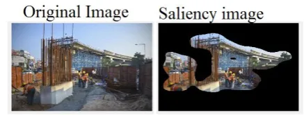
The input image is first segmented using a quaternion based saliency map technique. Saliency maps are used for segmentation due to the fact that on a metro site, the constructed area and the equipment’s are the most visually appealing parts. The saliency map does a perfect job at extracting those parts from the image, and removing all the other unwanted regions from it. It can be seen from figure 2 that the saliency map extracts all the visually important information from the imagery

Figure 2. Results of Saliency map on a sample image

The saliency map algorithm, divides the image into R, G and B components, then applies a quaternion technique to represent the pixels in a 3D region. These pixels are then smoothened using a gaussian filter. The smoothened pixels are given to an entropy calculation block, which finds out the best energy pixels from the given set. The best energy pixels when combined, form the rough saliency map. This rough saliency map is again smoothened using the gaussian filter, and then given to a border cutting and center biasing block, which removes all the unwanted edges from the image and produces a final saliency map image, as shown in figure 2. We tested the algorithm on various images and found that it gives almost optimum results for most of them.

viewing the picture as a whole, confusing saliency detection. These examples are not special, and exhibit one common problem – that is, when objects contain salient smalls cale patterns, saliency could generally be misled by their complexity. Given texture existing in many natural images, this problem cannot be escaped. It easily turns extracting salient objects to finding cluttered fragments of local details, complicating detection and making results not usable in, for example, object recognition, where connected regions with reasonable sizes are favored. Aiming to solve this notorious and universal problem, we propose a hierarchical model, to analyze saliency cues from multiple levels of structure, and then integrate them to infer the final saliency map. Our model finds foundation from studies in psychology, which show the selection process in human attention system operates from more than one levels, and the interaction between levels is more complex than a feed-forward scheme. With our multi-level analysis and hierarchical inference, the model is able to deal with salient small-scale structure, so that salient objects are labeled more uniformly.

Feature extraction using color map and edge map techniques

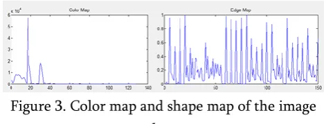
Color map or extended histogram map is obtained by plotting the quantized color levels on X axis and the number of pixels matching the quantized color level on the Y axis. The obtained graph describes the color variation of the image and thus is used to describe the image during classification stage. The color map resembles to the gray level histogram of the image with one minor difference, that the color map quantizes the R, G and B components of the image before counting them, while the histogram directly counts the pixels belonging to a particular gray level and plots them. This ensures that all the color components of the image are taken into consideration by the descriptor.

While color map describes the color of the image, the extended edge map describes the edge variation in the image. To find the edge map, the image is first converted into binary, and then canny edge detector is applied to it. The original RGB image is quantized same as in the color map. The locations of the edges are observed, and the probability of occurrence edge on a particular quantized image level is plotted against the quantized pixels in order to evaluate the edge map of the image. The edge map is used to define the shape variation in the image and is a very useful and distinctive feature for any image classification system. These 2 features combined together can describe the image in terms of color and shape, and are demonstrated in figure 3 for the image under test.

Figure 3. Color map and shape map of the image under test

Consider the following question: pick any pixel P1 of color Ci in the image I, at distance k away from p1 pick another pixel p2, what is the probability that p2 is also of color Ci. It’s easy to know, the histogram of these two images are exactly same. We can’t tell these two images from each other from the histogram. The auto-correlogram integrates the color information and the space information. For each pixel in the image, the auto-correlogram method needs to go through all the neighbors of that pixel. So the computation complexity is O(k*N^2), where k is the number of neighbor pixels, which is depended on the distance selection. The computation complexity grows fast when the distance k is large. But it’s also linear to the size of the image.

Feature extraction using SuRF and MSER features

Computing features consists of detecting SURF interest points and MSER interest regions, then calculating the corresponding feature descriptors. Furthermore, since SURF and MSER work only on grey scale images color correlograms and ICCV are utilized to extract color features. SURF was first introduced in (Bay et al., 2008) as an innovative interest point detector and descriptor that is scale and rotation invariant, as well as its computation, is considerably very fast. SURF generates a set of interesting points for each image along with a set of 64- dimensional descriptors for each interest point. On the other hand, Matas et al. (2002) presented MSER as an affine invariant feature detector. MSER detects image regions that are covariant to image transformation, which are then used as interest regions for computing the descriptors. The descriptor is computed using SURF. Thus, there is a set of interesting region for each image. These regions have a set of key points, which are presented by 64-dimensional descriptors for each. To extract the color features color correlograms (Huang et al., 1997) and ICCV (Chen et al., 2007) are implemented. Color correlograms feature represents the correlation of colors in an image as a function of their spatial

distances, it captures not just the distribution of colors of pixels as color histogram, but also captures their spatial information in the images. The color correlograms size hinges on the number of quantized colors exploited for feature extraction. In this study, we consider the RGB color model and implemented 64 quantized colors with two distances. Hence, the size of the correlograms feature vector is 2×64. ICCV divides the color histogram into two components: A coherent component that contains pixels that are spatially connected and a non-coherent component that comprises pixels that are detached. Furthermore, it contains more spatial information than that of traditional color coherence vector, which improves its performance without much-added computing work (Chen et al., 2007). In this exertion, the ICCV feature vector is formed of 64 coherence pairs, each pair provides the number of coherent and noncoherent pixels of a specific color in the RGB space. Thus, the size of ICCV is 2×64. The obtained feature vectors from the images in each training set of each class in the database are combined and portrayed as a multidimensional feature vector. BoVW is inspired directly from the bag-of-words methodology, which is trendy and extensively applied technique for text retrieval. In bag-of-words methodology, a document is characterized by a set of distinctive keywords. A BoVW is a counting vector of the occurrence frequency of a vocabulary of local visual features (Liu, 2013; Bosch et al., 2007). To distil the BoVW characteristic from images, the extracted local descriptors are quantized into visual words to form the visual dictionary. Hence, each image is portrayed as a vector of words like one document. Then, the occurrences of each individual word in the dictionary of each image are obtained in order to build the BoVW (histogram of words).

III.

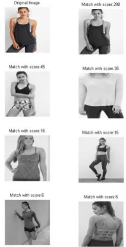
images collected from the Berkley Fashion Database. These images were first trained in the system, and then evaluation was performed on each of the input images. The following figures show some results obtained from the system,

Figure 1. Results for dress type 1

From figure 1, it is inherent that the fashion trends which match the given input color image, are matching with the output images. The designers and fashion crafters can use this information in order to evaluate the overall system and show the users the trends which match the given input dress type.

Figure 2, 3 and 4 also demonstrate similar results for different dress types,

Figure 2, 3 and 4. Different results for different dress types

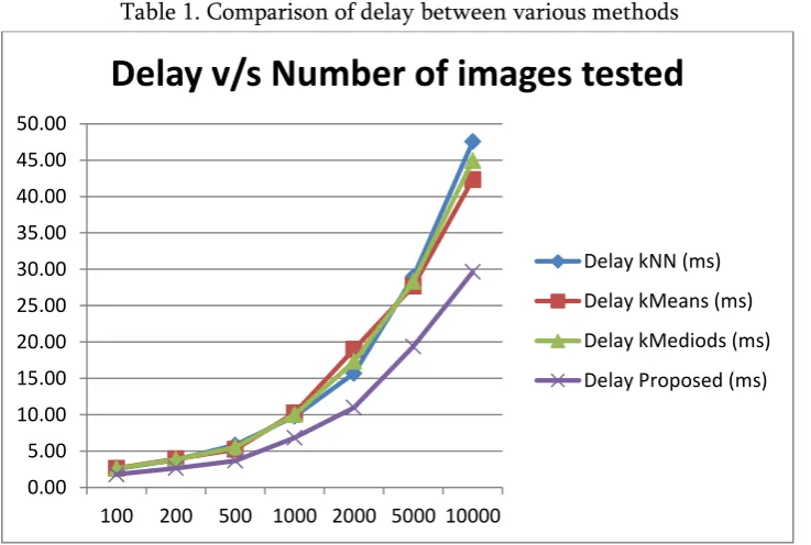
is better as compared to kNN, kMediods and kMeans clustering techniques. Number of

images tested

Delay kNN (ms)

Delay kMeans (ms)

Delay kMediods (ms)

Delay Proposed (ms)

100 2.58 2.63 2.61 1.81

200 3.79 3.93 3.86 2.65

500 5.82 5.23 5.53 3.66

1000 9.78 10.25 10.02 6.85

2000 15.69 18.99 17.34 10.98

5000 28.96 27.68 28.32 19.38

10000 47.53 42.33 44.93 29.63

Table 1. Comparison of delay between various methods

Figure 5. Performance comparison graph for delay

Similar comparison was made for precision of the system, and results are shown as follows

Number of images tested

Precision kNN (%)

Precision kMeans (%)

Precision kMediods (%)

Precision Proposed (%)

100 82.50 85.30 86.20 93.60

200 83.60 85.90 87.10 94.20

500 83.90 86.60 87.80 94.80

1000 84.73 87.23 88.63 95.40

2000 85.43 87.88 89.43 96.00

5000 86.13 88.53 90.23 96.60

10000 86.83 89.18 91.03 97.20

Table 1. Comparison of precision between various methods

0.00 5.00 10.00 15.00 20.00 25.00 30.00 35.00 40.00 45.00 50.00

100 200 500 1000 2000 5000 10000

Delay v/s Number of images tested

Figure 6. Performance comparison graph for precision From the above comparison, we can conclude that the developed algorithm is 10% faster when compared to other standard techniques and is more than 20% more accurate in terms of precision of the system.

IV.

CONCLUSION

From the results, we can conclude that the developed system can evaluate the images more than 10% faster as compared to the existing implementations, and has 20% better accuracy. This accuracy can further be improved using machine learning and artificial intelligence based techniques. The current technique uses multiple features like SuRF, MSER and color & edge maps in order to evaluate the content based retrieval of fashion components using correlation based matching, but this technique can be improved using multiple machine learning classifiers and artificial intelligence techniques like deepnets, Q-Learning and regression based learning mechanisms. Researchers can also improve the feature extraction techniques in the system in order to improve the overall quality of detection.

V.

REFERENCES

[1]. Z Al-Halah, R. Stiefelhagen, and K. Grauman. Fashion forward: Forecasting visual style in fashion. In ICCV, 2017.

[2]. L Bossard, M. Dantone, C. Leistner, C. Wengert, T. Quack, and L. Van Gool. Apparel classification with style. In ACCV, 2012.

[3]. J Carbonell and J. Goldstein. The use of mmr, diversitybased reranking for reordering documents and producing summaries. In ACM SIGIR, 1998. [4]. H Chen, A. Gallagher, and B. Girod. Describing

clothing by semantic attributes. In ECCV, 2012. [5]. J Chen, J. Zhu, Z. Wang, X. Zheng, and B. Zhang.

Scalable inference for logistic-normal topic models. In Advances in Neural Information Processing Systems (NIPS), 2013.

[6]. Q Chen, J. Huang, R. Feris, L. M. Brown, J. Dong, and S. Yan. Deep domain adaptation for describing people based on fine-grained clothing attributes. In CVPR, 2015.

[7]. J Deng, W. Dong, R. Socher, L.-J. Li, K. Li, and L. Fei-Fei. Imagenet: A Large-Scale Hierarchical Image Database. In CVPR, 2009.

[8]. W Di, C. Wah, A. Bhardwaj, R. Piramuthu, and N. Sundaresan. Style finder: Fine-grained clothing style detection and retrieval. In CVPR, 2013.

[9]. Q Dong, S. Gong, and X. Zhu. Multi-task curriculum transfer deep learning of clothing attributes. In WACV. IEEE, 2017.

[10]. K. El-Arini, G. Veda, D. Shahaf, and C. Guestrin. Turning down the noise in the blogosphere. In ACM SIGKDD, 2009.

[11]. J. Fu, J. Wang, Z. Li, M. Xu, and H. Lu. Efficient clothing retrieval with semantic-preserving visual phrases. In ACCV, 2012.

[12]. B. Gong, W. Chao, K. Grauman, and F. Sha. Diverse sequential subset selection for supervised video summarization. In NIPS, 2014.

[13]. C. Guestrin, A. Krause, and A. Singh. Near-optimal sensor placements in gaussian processes. In ICML, 2005.

[14]. X. Han, Z. Wu, Y.-G. Jiang, and L. S. Davis. Learning fashion compatibility with bidirectional lstms. ACM MM, 2017.

[15]. K. He, X. Zhang, S. Ren, and J. Sun. Deep residual learning for image recognition. In CVPR, 2016. [16]. R. He, C. Packer, and J. McAuley. Learning

compatibility across categories for heterogeneous item recommendation. In ICDM, 2016.

[17]. W.-L. Hsiao and K. Grauman. Learning the latent “look”: Unsupervised discovery of a style-coherent embedding from fashion images. In ICCV, 2017.

[18]. Y. Hu, X. Yi, and L. Davis. Collaborative fashion