Shape Representation in Primate Visual Area 4 and Inferotemporal Cortex

(1)

University of Pennsylvania

ScholarlyCommons

Publicly Accessible Penn Dissertations

Spring 5-17-2010

Shape Representation in Primate Visual Area 4 and

Inferotemporal Cortex

Thomas M. Murphy

University of Pennsylvania, [email protected]

Follow this and additional works at:http://repository.upenn.edu/edissertations Part of theBiomedical Engineering and Bioengineering Commons

Recommended Citation

Murphy, Thomas M., "Shape Representation in Primate Visual Area 4 and Inferotemporal Cortex" (2010).Publicly Accessible Penn Dissertations. 417.

(2)

Shape Representation in Primate Visual Area 4 and Inferotemporal Cortex

Abstract

The representation of contour shape is an essential component of object recognition, but the cortical mechanisms underlying it are incompletely understood, leaving it a fundamental open question in

neuroscience. Such an understanding would be useful theoretically as well as in developing computer vision and Brain-Computer Interface applications. We ask two fundamental questions: “How is contour shape represented in cortex and how can neural models and computer vision algorithms more closely approximate this?” We begin by analyzing the statistics of contour curvature variation and develop a measure of salience based upon the arc length over which it remains within a constrained range. We create a population of V4-like cells – responsive to a particular local contour conformation located at a specific position on an object’s boundary – and demonstrate high recognition accuracies classifying handwritten digits in the MNIST database and objects in the MPEG-7 Shape Silhouette database. We compare the performance of the cells to the “shape-context” representation (Belongie et al., 2002) and achieve roughly comparable recognition accuracies using a small test set. We analyze the relative contributions of various feature sensitivities to recognition accuracy and robustness to noise. Local curvature appears to be the most informative for shape recognition. We create a population of IT-like cells, which integrate specific information about the 2-D boundary shapes of multiple contour fragments, and evaluate its performance on a set of real images as a function of the V4 cell inputs. We determine the sub-population of cells that are most effective at identifying a particular category. We classify based upon cell population response and obtain very good results. We use the Morris-Lecar neuronal model to more realistically illustrate the previously explored shape representation pathway in V4 – IT. We demonstrate recognition using spatiotemporal patterns within a winnerless

competition network with FitzHugh-Nagumo model neurons. Finally, we use the Izhikevich neuronal model to produce an enhanced response in IT, correlated with recognition, via gamma synchronization in V4. Our results support the hypothesis that the response properties of V4 and IT cells, as well as our computer models of them, function as robust shape descriptors in the object recognition process.

Degree Type

Dissertation

Degree Name

Doctor of Philosophy (PhD)

Graduate Group

Bioengineering

First Advisor

Brian Litt, M.D.

Second Advisor

(3)

Third Advisor

Gershon Buchsbaum, Ph.D.

Keywords

shape representation, object recognition, IT, inferotemporal cortex, V4, macaque

Subject Categories

(4)

SHAPE REPRESENTATION IN PRIMATE VISUAL AREA 4 AND INFEROTEMPORAL CORTEX

Thomas Michael Murphy

A DISSERTATION

in

Bioengineering

Presented to the Faculties of the University of Pennsylvania

in Partial Fulfillment of the Requirements for the Degree of Doctor of Philosophy

2010

______________________________ Brian Litt, M.D.

Supervisor of Dissertation

______________________________ Susan Margulies, Ph.D. Graduate Group Chairperson

Leif H. Finkel, M.D., Ph.D. Advisor

(5)

Shape Representation in Primate Visual Area 4 and Inferotemporal Cortex

COPYRIGHT

2010

(6)

Dedication

For Louise & Leif

(7)

Acknowledgment

Thanks to my friends and colleagues throughout the university, particularly in the Finkel and Litt labs, for innumerable useful and enjoyable conversations.

Thanks to Brian for guidance and support during the most trying of times.

Thanks to Gershon, Larry, Jianbo and Bill for helpful advice throughout this process.

Thanks to Maciej for encouragement and feedback at critical junctures.

Thanks to Leif for inspiration.

(8)

ABSTRACT

SHAPE REPRESENTATION IN PRIMATE VISUAL AREA 4 AND INFEROTEMPORAL CORTEX

Thomas Michael Murphy

Brian Litt, M.D.

The representation of contour shape is an essential component of object recognition, but

the cortical mechanisms underlying it are incompletely understood, leaving it a

fundamental open question in neuroscience. Such an understanding would be useful

theoretically as well as in developing computer vision and Brain-Computer Interface

applications. We ask two fundamental questions: “How is contour shape represented in

cortex and how can neural models and computer vision algorithms more closely

approximate this?” We begin by analyzing the statistics of contour curvature variation

and develop a measure of salience based upon the arc length over which it remains within

a constrained range. We create a population of V4-like cells – responsive to a particular

local contour conformation located at a specific position on an object’s boundary – and

demonstrate high recognition accuracies classifying handwritten digits in the MNIST

database and objects in the MPEG-7 Shape Silhouette database. We compare the

performance of the cells to the “shape-context” representation (Belongie et al., 2002) and

achieve roughly comparable recognition accuracies using a small test set. We analyze the

(9)

recognition. We create a population of IT-like cells, which integrate specific information

about the 2-D boundary shapes of multiple contour fragments, and evaluate its

performance on a set of real images as a function of the V4 cell inputs. We determine the

sub-population of cells that are most effective at identifying a particular category. We

classify based upon cell population response and obtain very good results. We use the

Morris-Lecar neuronal model to more realistically illustrate the previously explored

shape representation pathway in V4 – IT. We demonstrate recognition using

spatiotemporal patterns within a winnerless competition network with FitzHugh-Nagumo

model neurons. Finally, we use the Izhikevich neuronal model to produce an enhanced

response in IT, correlated with recognition, via gamma synchronization in V4. Our

results support the hypothesis that the response properties of V4 and IT cells, as well as

our computer models of them, function as robust shape descriptors in the object

(10)

List of Tables

Table 4.1 – Comparison of results

Table 4.2 – Summary of results for the entire 10,000 digit images from the MNIST “Test Set” database

(14)

List of Illustrations

Figure 3.1 – Shashua & Ullman image

Figure 3.2 – Method of calculation of curvature at each pixel Figure 3.3 – Threshold at 45% of curvature range

Figure 3.4 – Threshold at 35% of curvature range Figure 3.5 – Threshold at 15% of curvature range

Figure 3.6 – Gaussian model of circle vs. background curvatures Figure 4.1 – Curvature histograms

Figure 4.2 – Corresponding points, matching costs, and sum of squared differences Figure 4.3 – x, y, tangent, and curvature values

Figure 4.4 – Segmentation

Figure 4.5 – 2-dimensional Gaussian population responses

Figure 4.6 – 4-dimensional Gaussian responses, with arbitrarily assigned clockwise- and counterclockwise-adjacent curvatures

Figure 4.7 – Matching matrix Figure 4.8 – Misclassified digit Figure 4.9 – Matching matrix

Figure 4.10 – Parameter comparisons Figure 4.11 – Parameter comparisons Figure 4.12 – Parameter comparisons Figure 4.13 – Feature inclusion summary Figure 4.14 – Noisy features

Figure 4.15 – Noisy features

Figure 4.16 – Matching matrix for the entire 10,000 digit images from the MNIST “Test Set” database

Figure 4.17 – MPEG-7 Shape Silhouette database

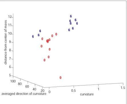
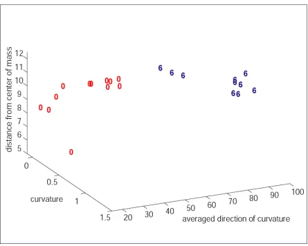
Figure 4.18 – Dimensional inseparability of segment features of "0" and "6" images Figure 4.19 – Dimensional separability of segment features of "0" and "6" images Figure 4.20 – 1 o'clock segments

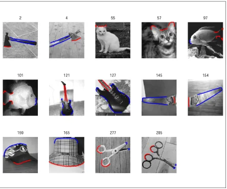
Figure 5.1 – Example images

Figure 5.2 – Parts, segments, curvatures, directions, etc., for one image Figure 5.3 – Image normalization

Figure 5.4 – Feature vector values for one image Figure 5.5 – Matching matrix

Figure 5.6 – Normalized average-to-average Earth Mover’s Distance Figure 5.7 – Percentage of total Earth Mover’s Distance comparison Figure 5.8 – Iso-curvature segments

(15)

Figure 5.11 – Normalized distribution of all parameter values for all cells Figure 5.12 – Gaussian constituents and iso-curvature segments

Figure 5.13 – Gaussian constituents

Figure 5.14 – Histogram of IT cell responses

Figure 5.15 – Response of four cells from the population to each image Figure 5.16 – Principal Components Analysis (PCA)

Figure 5.17 – Biplot Figure 5.18 – Pareto chart Figure 5.19 – Shepard plot

Figure 5.20 – Three-dimensional non-classical non-metric multidimensional scaling (MDS) analysis

Figure 5.21 – Hypothesis of no correlation

Figure 5.22 – Cell population responses to each image in two categories Figure 5.23 – Decision tree for classification

Figure 5.24 – Responses of six alternatively-constructed cells to each image Figure 5.25 – Response contributions of one cell

Figure 5.26 – Responses of six alternatively-constructed cells to each image Figure 5.27 – Response contributions of one cell

Figure 5.28 – Iso-curvature segments’ contributions to Gaussian constituents’ responses Figure 5.29 – Sub-populations

Figure 5.30 – Accuracy

Figure 6.1 – Morris-Lecar model validation

Figure 6.2 – Morris-Lecar cell’s response to selected images Figure 6.3 – Morris-Lecar cell’s response to each image

Figure 6.4 – Winnerless competition network topography with 9 neurons Figure 6.5 – FitzHugh-Nagumo model

Figure 6.6 – FitzHugh-Nagumo neuron within a winnerless competition network Figure 6.7 – FitzHugh-Nagumo neuron within a winnerless competition network Figure 6.8 – Izhikevich model validation

Figure 6.9 – Izhikevich network without feedback Figure 6.10 – Izhikevich network with feedback

(16)

Chapter 1

General Introduction

1.1 The Ventral Stream and Models of Object

Recognition

(17)

salience upon objects, although their relative contributions to overall salience and manners of integration remain unclear.

Ullman has proposed the idea that salience is a global property that integrates the Gestalt factors across an entire object (Shashua and Ullman, 1988; Ullman, 1996). Closure is itself a global property (Yen and Finkel, 1998), and Kovács and Julesz have shown, using roughly circular contours, that closure leads to a marked increase in salience (Kovács and Julesz, 1993). In Ullman’s original algorithm, salience is determined by the length, continuity and curvature of the contour. Long, smooth contours with little change of curvature and no gaps are calculated to be the most salient. Curvature covariation has been investigated (Chapter 3), and in a detailed study of Ullman’s methodology, Alter and Basri have found that, for many images, their algorithm robustly predicted salience values in accord with human perception (Alter and Basri, 1996). In this dissertation, we consider closed 2-dimensional bounding contours primarily, and concern ourselves with downstream functionalities, namely representation and recognition.

(18)

significant amount of research attention. Virtually all visual sensory information in the ventral pathway passes through extrastriate area V4 on its way to the inferotemporal areas (Ungerleider and Mishkin, 1982), with V4 receiving inputs from visual area 2 (V2) and providing the major source of input to IT (Felleman and Van Essen, 1987; Felleman and Van Essen, 1991).

Selectivity for simple dimensions, such as orientation, spatial frequency, length and width, has been demonstrated in V4 (Desimone and Schein, 1987), but these properties have also been found in earlier stages of form processing, such as area V1. The Van Essen group, however, has been successful in finding selectivities in V4, thought to be form-related, that have not been found in earlier stages. They have found that nearly all V4 neurons, while biased towards polar and hyperbolic stimuli over Cartesian stimuli, convey information about all three stimulus classes, with most having tuning curves in multiple classes (Gallant et al., 1996). This, along with their positional invariance, perhaps suggests that V4 cells are neither simple feature detectors nor simple filters, but rather nonlinear filters broadly tuned along several form-related dimensions. V4 cells responsive to polar stimuli could facilitate the perception of curvature, an important feature in natural image understanding, as well as mediate view invariance.

(19)

this, may be present. Object-centered coordinates such as these within a local reference frame could yield translation and scale invariance, desirable in any recognition system, biological or artificial. This is analogous and consistent with the idea of human navigation being largely dependent upon a continuously updated egocentric representation of object locations, with a lesser dependence upon an enduring allocentric map of environmental shape (Wang and Spelke, 2000). Note that a neural code of human spatial navigation based on cells that respond at specific locations and cells that respond to views of landmarks has been identified in the hippocampus and parahippocampal region (Ekstrom et al., 2003).

Research by Connor and colleagues has identified cells in area V4 that are selective for both the local shape and the global position of segments of object borders, with most cells strongly responsive to a particular type of boundary conformation at a specific position within a larger shape (Pasupathy and Connor, 2001; Pasupathy and Connor, 2002). Specifically, these neurons are selective for both the magnitude and direction of curvature of a stimulus, and individual V4 cells appear to encode moderately complex boundary information at specific locations within larger shapes.

(20)

individual cells encode smaller parts of larger objects) (Pasupathy and Connor, 2001). If shapes are represented as combinations of primitive features then shape recognition could be seen as a hierarchical process. With areas V2 and V4 selective both for the magnitude and direction of curvature, area V1 could provide the input to a population of local curvature detectors while area V4 could perform global matching between the curvature detectors. It is conceivable that feedback from area V4 to area V1 provides some top-down control of salience. A number of studies have proposed neural and computational mechanisms for computing curvature (Dobbins et al., 1989). These lower level curvature calculations are consistent with mechanisms, such as end-stopping, available in primary visual cortex.

(21)

The surprising finding by von der Heydt and associates – that a majority of cells in V2 and V4, and a smaller number of cells in V1, carry information about how local features belong to objects – is significant. Specifically, these neurons were seen to code the side to which a border in a figure belongs (Zhou et al., 2000). This response was seen to be generated within the visual cortex, not projected down from higher levels, and clearly represents global image context integration. Perception tends to assign contrast borders to objects, according to the Gestalt psychologists, and the von der Heydt results show that this is accomplished at an earlier cortical level than previously thought.

(22)

Both the von der Heydt as well as the Hegdé / Van Essen results give credibility to a hierarchical feedforward flow of visual information model, from V1 / V2 to V4 to IT, to support visual form processing. These results can be considered in the context of information theory, with quantification of the amount of stimulus information carried by neural responses (Borst and Theunissen, 1999).

(23)

Feedback pathways for top-down modulation of responses and support of learning may also be incorporated.

The work by Hinkle and associates provides some insights into the global significance of area V4. The finding that stereoscopic disparity tuning (conventionally associated with the dorsal pathway) is prevalent in area V4 positions it as a major source of disparity information for IT and emphasizes the importance of stereoscopic depth cues in the ventral pathway (Hinkle and Connor, 2001). It also suggests that 3-dimensional shape information is processed in V4 based on these cues. A bias towards certain disparities has also been observed, possibly reflecting the ventral pathway’s particular emphasis on foreground objects or parts of objects projecting towards the viewer. The finding that neurons in area V4 are tuned for 3-dimensional orientation (Hinkle and Connor, 2002) supports these ideas and further suggests that the initial stages of shape analysis utilize depth cues. Three-dimensional orientation tuning facilitates the computationally difficult 3-dimensional position invariance and is compatible with both viewpoint-invariant and viewpoint-dependent models.

(24)

(Hinkle and Connor, 2001), and complex spatial patterns (Gallant et al., 1996). Extrastriate cells show selectivities to several aspects of form (Gallant et al., 1996) and border ownership (Zhou, Friedman and von der Heydt, 2000). In addition, V4 cell receptive field properties are strongly modulated by attention (Reynolds and Desimone, 2003; Bichot, Rossi and Desimone, 2005; McAdams and Maunsell, 2000; Motter, 1994; Connor et al., 1997), and the presence of a small feature within the large receptive field can drive cellular response.

(25)

An intriguing idea has emerged that suggests that area V4, as a key stage in a network of cortical and subcortical areas working in concert, contains a retinotopic salience map that guides saccadic eye movements during free viewing (Mazer and Gallant, 2003). It is seen that bottom-up, visually driven activity in V4 predicts the direction of subsequent saccades and is modulated by top-down, feature attention-related signals. Information about the spatial distribution of activity in V4 could be used in downstream areas to guide subsequent exploratory eye movements toward interesting positions in the visual field. Future efforts might include modeling the significant contribution of top-down information from higher cortical areas. This not only can localize the regions of interest, but also can make adjustments to the iso-curvature segments as well.

(26)

hierarchical feedforward implementation, with IT input originating in V4. It is related to the fragment-based approach of Ullman and colleagues. Here, fragments (contour segments producing responses in V4) are the component building blocks used to represent a large variety of objects belonging to a common class (Ullman et al., 2001).

(27)

stable, map of shape selectivity in IT that is largely independent of object class familiarity and behavioral task (Op de Beeck et al., 2008). McMahon and Olson have reported that the influences of shape and color sum linearly in most IT neurons, with neither conjunction selectivity nor a specialized feature binding process necessary for representation (McMahon and Olson, 2009).

As with V4, a complete model of IT might have to incorporate 3-dimensional information. Yamane and colleagues have found evidence in IT for an explicit neural code for complex 3-dimensional shape, with widespread tuning for the spatial configurations of surface fragments (Yamane et al., 2006; Yamane et al., 2008). Sereno and colleagues have suggested that 3-dimensional shape representations are highly localized, yet widely distributed in occipital, temporal, parietal and frontal cortices, with distributed networks intersecting both “what” and “where” processing streams (Sereno et al., 2002).

(28)

high-level information by using class-specific criteria. Another technique, useful in segmenting an image into foreground and background (Yu and Shi, 2003), employs parallel processes: one for low-level pixel grouping for feature saliency and another for high-level patch grouping for object familiarity.

The state-of-the-art category-level recognition system of Malik and colleagues (Belongie

et al., 2002) provides a shape description based on the distances between all pairs of points on the object’s bounding contour. Shape context log-polar histograms are computed for each point on the contour. The collection of histograms fully characterizes each shape. Malik solves the correspondence problem between two shapes using optimal assignment. He estimates the aligning transform using these correspondences and regularized thin-plate splines. Finally, he measures similarity between the shapes as a function of matching errors between corresponding points and aligning transform magnitude.

(29)

A future successful model of V4 would have to incorporate other findings as well. For instance, the position and variability of the color center and retinotopic organization within V4 has been investigated (McKeefry and Zeki, 1997). Also, direction-of-motion selectivity after adaptation has been confirmed (Tolias et al., 2005) and has great significance.

(30)

1.2 Computational Neuroscience – Necessity and

Benefits

The somewhat controversial nature of computational neuronal modeling is exemplified by the recent “cat brain” debate (Adee, 2009) between Dharmendra Modha, a computer scientist on DARPA’s SyNAPSE project who presented a simulation that his team claimed approached the scale of a cat’s brain, and Henry Markram, a neuroscientist who claimed that the simulation was a hoax, calling into question the legitimacy of brain simulation research. Modha’s position was that the simulation was not a cat brain, but rather on the scale of a cat’s brain, in terms of the number of neurons and synapses. Markram objected to the impoverished detail in the simulation’s point neurons and regarded it as trivial.

We feel that the acquisition of physiological and anatomical data alone is insufficient for a complete understanding of neural processing. To learn how the brain works, experimental studies of animal and human nervous systems must be coupled with computational brain models. At this stage, neuroscience requires a quantitative framework to integrate and manage its enormous amount of experimental data. Computational neuroscience can provide this.

(31)

far exceed what is biologically practical. A model provides access to mechanisms with levels of sensitivity and specificity that are unavailable experimentally, as well as the ability to record all parameters simultaneously. Computational protocols may be run repeatedly, with little or no preparatory work, without concern for loss or sacrifice of specimens.

It is reasonable to think that a sufficiently detailed neuronal model, imbedded within a realistic network, will produce realistic behavior. A good model should be able to reproduce experimental results and it should allow us to generate predictions and test hypotheses at the appropriate level of detail. It even has the capacity to contradict experimental expectations.

Simplified models may sacrifice biological accuracy for computational efficiency, but models do not have to be perfect to be useful. Therefore, we create models with as much physiological and anatomical fidelity as is available to us in the published literature, while remaining tractable. This represents a compromise between the requirements of simple computation and biological realism. We must, however, understand the simplifications if we are to understand the connections between our computational models and nature.

(32)

some assumptions made to fill knowledge gaps may be incorrect. None of these shortcomings are insurmountable.

We feel that computational neuroscience should ideally augment, guide and complement experimental neuroscience, rather than replace it. This dual approach should provide intuitions and a deeper understanding for both sub-disciplines. Most importantly, computational simulations might lead to interesting and novel insights and unexpected results that can later be validated experimentally.

1.3 MATLAB Models

We have used GENESIS (see http://genesis-sim.org/), NEURON (see

http://www.neuron.yale.edu/neuron/), Java (see http://java.sun.com/), python (see

http://www.python.org/), etc., to create computational neural models.

Our primary tool, however, is MATLAB. Its modular design, high-level code, flexible interface options, device independence, numerical algorithms and data visualization capabilities make it ideal for our purposes. Unsatisfactory execution time has simply never been an issue for us.

With many third-party toolboxes available (such as Bayes Net Toolbox for Matlab:

(33)

choice for computational neuroscientists, as well as scientists and engineers in general, worldwide.

(34)

Chapter 2

Research Overview

2.1 Chapter Contents

(35)

these results in view of Rosenholtz’s (Rosenholtz, 1999) model of salience as a statistical measure of outliers from a population. In addition, we speculate on the visual cortical mechanisms in striate and extrastriate cortex required to carry out salience measurements on this class of images. A portion of this material has been previously published (Murphy et al., 2003).

(36)

the contour segment from object center, and modulatory effect of adjacent contour regions. Among these, local curvature appears to be the most informative variable for shape recognition. Our results support the hypothesis that V4 cells function as robust shape descriptors in the early stages of object recognition. A portion of this material has been previously published (Murphy and Finkel, 2007).

(37)

analysis and a 2-dimensional and 3-dimensional non-classical non-metric multidimensional scaling analysis. We find the correlation coefficients of the observations (cell responses) and variables (images) and determine the sub-population of cells that are most effective at identifying a particular category. We use a support vector machine, as well as a tree-based model, for classification based upon cell population response. In general, we obtain very good results across a wide range of parameter values and implementation strategies, comparable to those obtained previously with the digit database. Our results suggest that curvature- and position-sensitive units, as described by Brincat and Connor in IT, can function as robust shape descriptors.

(38)

onset of synchronization. Our results suggest that realistic biological models of cells with curvature- and position-sensitive response properties, as described by Pasupathy and Connor in V4 and Brincat and Connor in IT, can function as robust shape descriptors.

We summarize our results in Chapter 7 and discuss future steps in Chapter 8.

2.2 Acknowledgements

This work was supported by the DoD Multidisciplinary University Research Initiative (MURI) program administered by the Office of Naval Research under Grant N00014-01-1-0625 as well as grant 9873463 from the NSF KDI program.

The work was also supported by generous Research Fellowships from the University of Pennsylvania.

2.3 Motivation, Personal Objectives and Research

Goals

(39)

handwritten digits. We sought to develop a model of IT response based on V4 inputs and evaluate the performance of an IT population on a set of real images. We sought to investigate the recognition performance within the IT network as a function of the number of V4 subunits and their nonlinear combinations. Finally we sought to explore the connections between our model and current psychological models of object categorization. (Incidentally, all of these objectives have been accomplished.)

Perhaps, though, our motivation and goals should be expanded slightly.

The representation of contour shape is an essential component of object recognition, but the cortical mechanisms underlying shape analysis and object recognition are incompletely understood, leaving it a fundamental open question in neuroscience. We hope to approach such a neurobiological understanding, which would be useful theoretically as well as in developing or improving computer vision and Brain-Computer Interface (BCI) methodologies and applications.

(40)

We ask two fundamental questions: “How is contour shape represented in cortex and how can neural models and computer vision algorithms more closely approximate this?” Our primary objective is to determine why the response properties of V4 and IT cells (i.e., their receptive fields), and in particular their sensitivities to curvatures and contour positions, are useful. We hope to establish a clear connection between a computer model of a recognition system and known cortical constructs within a biologically realistic network architecture.

(41)

Chapter 3

Curvature Covariation as a Factor in

Perceptual Salience

3.1 Introduction

(42)

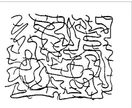
As Ullman pointed out, salience is a global property that integrates the Gestalt factors across an entire object (Shashua and Ullman, 1988; Ullman, 1996). In Figure 3.1, taken from Ullman’s original paper, the three circular contours pop out and are more salient than the background squiggles. We are interested, in this paper, in understanding quantitatively what factors render the circles salient.

One Gestalt factor that distinguishes the circular contours from the background is closure. Closure is itself a global property (Yen and Finkel, 1998), and Kovács and Julesz have shown, using roughly circular contours, that closure leads to a marked increase in salience (Kovács and Julesz, 1993).

In Ullman’s original algorithm, salience was determined by the length, continuity, and curvature of the contour. Long, smooth contours with little change of curvature and no gaps are calculated to be most salient. In a detailed study of this algorithm, Alter and Basri found that, for many images, it robustly predicted salience values in accord with human perception (Alter and Basri, 1996). To our knowledge, a detailed analysis of the original Ullman image (Figure 3.1) has not been performed.

(43)

(44)

3.2 Methodology

By deliberate construction, the three closed contours in Figure 3.1 are physically similar to the background contours in terms of contrast, thickness, and range of orientations. The background squiggles are not all continuous, but terminate at the borders of the figure, forming three open contours. The closed contours are shorter (239, 244, 243 pixels) than the background contours (1238, 2011, 880 pixels), but it is not clear that the terminations of the background contours are perceptually significant.

An erosion algorithm was first employed to reduce image contours down to single-pixel widths (using the MATLAB bwmorph function). We were then able to decompose the image into closed and background contours and investigate each separately.

Orientations were computed using Freeman & Adelson’s G2 / H2 steerable filters (Freeman and Adelson, 1991). At locations where contours cross, we ascertained that the correct orientation was assigned to each contour.

(45)

Figure 3.2 – Method of calculation of curvature at each pixel. 1

5

7 2

3

4

9 8 6

curvature(5)

= 40% [(θ6 – θ4) / (s6 – 4)]

+ 30% [(θ7 – θ3) / (s7 – 3)]

+ 20% [(θ8 – θ2) / (s8 – 2)]

+ 10% [(θ9 – θ1) / (s9 – 1)]

(46)

angle subtraction formulas are corrected modulo 360° so that, for example, the difference between a 350° orientation and a 10° orientation is 20°, not 340°.

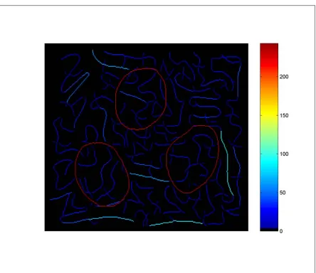
Once the curvature had been calculated at each pixel, cocircular segments were defined. A range (max curvature − min curvature) of curvature values for all contours was computed. Adjacent pixels on the same contour were deemed cocircular if the difference in their curvatures was below a set threshold, expressed as a percentage of this total curvature range.

All simulations were carried out using the MATLAB application development environment (version 6 R12) and the associated Image Processing Toolbox (version 3.1).

3.3 Results

We first investigated a number of technical image processing issues. We carried out the measurements with and without an initial contour-thickening step in an attempt to smooth out the thinned contours. Results were similar in both cases.

(47)

and the Euclidean distance between pixels for s (instead of the arc length). Both of these approaches were abandoned because of poor results. Other qualitatively poorer results were obtained using Gabor filters instead of steerable filters, performing calculations with overlapping segments of the contours, and mid-pixel averaging if greater than threshold. All of these techniques were subsequently dropped.

(48)

(49)

threshold the closed contours contain much longer stretches of cocircularity, compared to the background contours and cross-hatches.

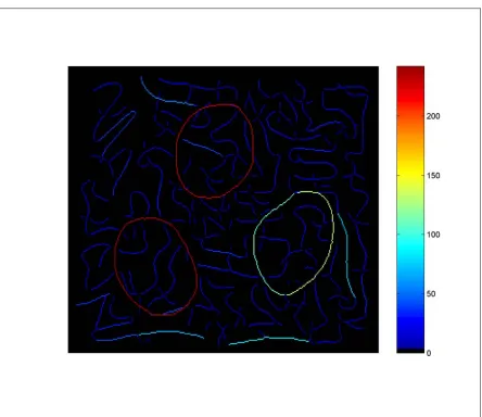
Figure 3.4 provides a similar computation when the threshold has been set to 35% of the maximal curvature range. This stricter threshold cuts down on the extent of contours conforming to the curvature constraints. Although the closed contours still contain longer segments meeting this criterion, the difference between the closed contours and background squiggles is less dramatic.

(50)

(51)

(52)

3.4 Discussion

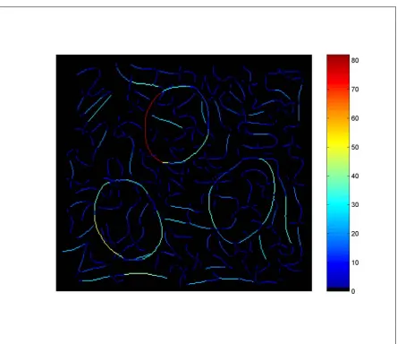
If curvature covariation is a factor in determining perceptual salience then Figure 3.3 argues that the circular contours should be more salient than the background. However, as Figures 3.4 and 3.5 demonstrate, the degree to which curvature covariation contributes to salience will depend upon the mechanisms and the scale over which curvature information is computed in visual cortex.

A number of studies have proposed neural and computational mechanisms for computing curvature (Dobbins et al., 1989). These lower level curvature calculations are consistent with mechanisms, such as end-stopping, available in primary visual cortex. At higher cortical levels, Van Essen, Connor and colleagues have shown that cells in areas V2 and V4 are selective both for the magnitude and direction of curvature (Hegdé and Van Essen, 2000; Pasupathy and Connor, 2001).

(53)

cells firing at the same rate is statistically unlikely. Thus, a set of connected V4 cells, each sensitive to magnitude and direction of curvature, which are coupled by horizontal connections, would rapidly synchronize in response to the circles, but to a much lesser degree to the background squiggles.

Salience depends upon the degree to which a target differs from the background. Rosenholtz (Rosenholtz, 1999) has proposed that a possible metric for salience is to consider the Mahalanobis distance between a target and the background. Thus, salient targets are those whose features are statistical outliers from the background population.

(54)

(55)

Area V4 is well situated to carry out computations of the type envisioned here. Connor and colleagues have found cells in macaque V4 that respond selectively to the magnitude and direction of curvature. V4 contains an extensive network of horizontal connections, which span significant portions of the visual field (Amir et al., 1993). Through these connections, possibly together with top-down information from higher temporal areas, V4 is thought to mediate contextual population-based interactions within the scene, such as those required in color constancy. Finally, V4 is known to play a critical role in determining salience. Lesions of V4 render animals incapable of detecting a less salient target in the presence of more salient distracters (Schiller, 1993).

3.5 Conclusion

(56)

Chapter 4

Shape Representation by a Network

of V4-like Cells

4.1 Introduction

The representation of contour shape is an essential component of object recognition. Human observers are exquisitely sensitive to changes in contour shape (Zana and Cavalcanti, 2005), and this capacity develops in early infancy (Norcia et al., 2005). However, the cortical mechanisms underlying shape analysis are incompletely understood.

(57)

Hegdé and Van Essen, 2003). In area V4, Pasupathy and Connor have described cells that are selective for a particular local shape configuration at a particular location on the contour (Pasupathy and Connor, 2001). For example, one neuron might prefer contours with a sharp concavity at the northwest corner; another unit might be selective for contours with a shallow convexity at the southernmost tip. The response of these cells is further modulated by the local contour configurations at neighboring locations on the contour. Thus, the unit preferring a sharp concavity at the NW corner might be potentiated by a sharp concavity located immediately clockwise along the contour, or suppressed by a convexity located immediately counterclockwise. Pasupathy and Connor have demonstrated that a population of such V4 units can provide a detailed description of the contour shape (Pasupathy and Connor, 2002).

(58)

digit “3”. This measure corresponds to that reportedly used by humans and monkeys in object classification (Sigala et al., 2002).

For the purposes of this study, we segment each contour into iso-curvature regions, and dedicate a V4-like unit to describing each region (its curvature, orientation, distance from object center, etc.). This approach is computationally tractable and connects conceptually to previous models of “parts-based” recognition (Biederman, 1987; Riesenhuber and Poggio, 1999; Ullman et al., 2001). However, there is no theoretical need for this initial segmentation stage – a large population of V4-like cells could describe overlapping regions of the contour in an over-complete representation.

(59)

We then test the performance of a population of V4-like cells on the MNIST database and the MPEG-7 Shape Silhouette database (Jeannin and Bober, 1999) and evaluate accuracy of classification. We analyze the contribution of sensitivities to different contour features (position, curvature at neighboring locations, etc.), and find that local curvature is the most critical component of the shape description.

4.2 Methodology

(60)

We next develop a stand-alone model of V4-like units to evaluate recognition performance. Simple image processing techniques are used to decompose the image into closed contours, each of which is analyzed independently (e.g., the inner and outer contours of a digit “9” (see Figure 4.2)). For each image, we extract contours using the numerical gradient, and determine a set of boundary points with oriented tangents. The result is a parametric description (x(t), y(t), and tangent(t)) of each contour. For each point along the contour, we compute its angle (0° − 360°) relative to and distance (in pixels) from the image’s center of mass. For consistency, we consider the contour’s points such that each contour begins at approximately 3 o’clock and proceeds counterclockwise.

Using the parametric forms x(t) and y(t), where 0 < t < L, L being the length of the curve, the curvature is given by:

κ(t) = ( ( dx/dt ) ( d2y/dt2 ) − ( d2x/dt2 ) ( dy/dt ) ) / ( ( dx/dt )2 + ( dy/dt )2 )3 / 2 .

(61)

Tsotsos (1997) is another technique for shape representation and recognition of objects. Based on smoothed multiscale curvature information and using a dynamic programming matching strategy, it is related to the CSS representation. Wuescher and Boyer’s (1991) formulation is something of a departure from Mokhtarian. Following their methodology, we convolve x(t) and y(t) with the derivative of a Gaussian to both smooth (regularize) and differentiate the functions. This results in the discrete curvature, parameterized by the Gaussian space constant:

κ(t, σ) = ( ( x(t) ∗ g′(t, σ) ) ( y(t) ∗ g′′(t, σ) ) −

( x(t) ∗ g′′(t, σ) ) ( y(t) ∗ g′(t, σ) ) ) / ( (x(t) * g′(t, σ) )2 + ( y(t) * g′(t, σ) )2 )3 / 2 ,

where

g(t, σ) = ( 1 / σ√2π ) exp( −t2 / 2σ2 _{) ,}

∗ is the convolution operator, and ′ is the differentiation operator.

(62)

κsquashed = ( 2.0 / ( 1 + exp( − 0.125 * κ ) ) ) − 1.0 .

We define the direction of curvature to be orthogonal to the tangent and to point towards the interior of the closed contour (Sajda and Finkel, 1995). It is computed using the orientation and inverse tangent.

Next, we segment each contour into iso-curvature regions using one of two methods. The first method is simplistic. We choose a standard size (in number of boundary points) for each region. Remaining points are evenly distributed. We choose a starting point on the contour (and therefore the starting point for each region) based upon the arrangement that yields the lowest average standard deviation of curvature for each region. Ideally, each iso-curvature segment has a zero standard deviation of curvature.

The second method, following Wuescher and Boyer’s (1991) curvature voting technique, considers segments of constant curvature (within a curvature tolerance tc) and segments

of rapidly changing curvature. Curvature is quantized into bins of a specified width (typically 1/2tc bins for every span of 0.10 in curvature), with peaks of the resulting

(63)

In the experiments described below, unless otherwise noted, a standard size (6 boundary points) for each iso-curvature region is chosen for segmentation. In addition, all contours are smoothed using a Gaussian function with a standard deviation of 2 pixels (a sigma value of 2).

For each iso-curvature segment of each image, we create feature vectors composed of various combinations of features chosen from the following: mean polar angle of contour region (e.g., 3 o’clock), mean curvature of the region, mean curvature of the clockwise adjacent region, mean curvature of the counterclockwise region, mean direction of curvature of the region, mean distance from the center of mass of the region, an indication of whether the region belongs to an inner vs. outer contour, and Gaussian averaged response of the region – the simulated response of a population of optimally positioned neurons across the curvature × position domain (see Figure 4.5 below). These features all have approximate neurobiological correlates in area V4 and other extrastriate areas (Desimone and Schein, 1987; Kobatake and Tanaka, 1994; Gallant et al., 1996; Pasupathy and Connor, 1999; Wilkinson et al., 2000; Zhou et al., 2000; Pasupathy and Connor, 2001; Pasupathy and Connor, 2002).

(64)

direction are employed). In our stand-alone framework of V4-like cells considered later, however, radial distance is one of the features that is examined. Secondly, “curvature contexts” are curvature / angular direction histograms and, like shape contexts, are computed with respect to every point on the contour. In our stand-alone framework of V4-like cells, however, curvature, angular direction, distance, etc., are computed with respect to the center of mass.

(65)

strongly with human color discrimination performance (i.e., distance approximately matches human perception of the differences between those colors) (Rubner et al., 2000; Wyszecki and Stiles, 1982; Tversky, 1977). Another advantage is that angle comparisons (for example, 358° is very close to 2°) can easily be handled.

All simulations were carried out using the MATLAB application development environment (version 7.3.0.267 R2006b) and the associated Image Processing Toolbox (version 5.3).

4.3 Results

(66)

(67)

untransformed correspondences between the points of each of the two images using optimal assignment (Figure 4.2 (A)). We then estimate the aligning transform between the two images using these correspondences and regularized thin-plate splines, measuring affine and matching costs (Figure 4.2 (B)). We present a representation of the first image after it has been warped into the second image (Figure 4.2 (E)). Finally, we compute the local sum of squared differences and average local sum of squared differences of this warping (Figure 4.2 (F)). Figure 4.2 (C,D,G,H) shows the same calculations for matching the two “9” digits from Figure 4.1.

We compare our results, after only one iteration, with those reported by Belongie and colleagues. For each numeric digit (“1’s”, “2’s”, etc.), two example images are randomly selected from our test set and compared to each other. We use Belongie’s shape context algorithm to compute the matching cost and SSD and compare the results to those obtained using curvature contexts. In both measures, lower values correspond to better matches. As shown in Table 4.1, “shape context” and “curvature context” shape representations achieve comparable recognition accuracies.

(68)

(69)

(70)

(71)

(72)

not required to align with a corresponding outer contour segment. In the bottom left image of Figure 4.4, for example, an inner contour segment begins at approximately 9 o’clock and ends at approximately 1 o’clock, while its corresponding outer contour segment begins at approximately 9 o’clock and ends at approximately 11 o’clock. The standard region size with lowest standard deviation method is shown in the left column. The constant curvature criterion method is shown in the right column, with open circles representing leftover portions. The segmentations appear qualitatively reasonable, approximating the expected results if the segmentation were performed “by eye”. For the images analyzed, we find that a segmentation region size of 6 pixels results in the greatest number of iso-curvature segments (21), while the curvature tolerance 0.2 results in the least (10). The degree to which the segmentation affects system performance is considered below.

(73)

(74)

panels. Note the visual dissimilarity between the left and right panels, again suggesting that some level of category discrimination is achieved in the curvature × position domain.

A 4-dimensional Gaussian tuning function (corresponding to Pasupathy and Connor’s (2001) Figure 3), for three adjacent boundary elements, is shown in Figure 4.6. Here, each individual surface plot represents the 2-dimensional Gaussian response of the central boundary element in the squashed curvature × angular position domain. The rows and columns of plots represent the modulatory effects of adjacent contour elements. The rows correspond to different arbitrarily assigned clockwise-adjacent curvatures, while the columns correspond to different arbitrarily assigned counterclockwise adjacent curvatures. A hypothetical cell responding optimally would exhibit strong tuning for a slight concavity towards the bottom of the image, flanked clockwise by a slight concavity and flanked counterclockwise by a slight convexity. The highlighted portion of the “2” digit exhibits these characteristics.

Recognition Performance of V4-like Units

(75)

(76)

image is compared to that of every other image, and the average distance from one digit to all other examples of the same digit is determined. This average (earth mover’s) distance calculation is motivated by human perceptual studies – evidence suggests that categorization is based on an average fit approximation to the class, rather than on exact matches to prototypes (Kahana and Sekuler, 2002). If an image’s lowest average distance is to a group of images representing the same digit then a match is said to have occurred. Otherwise, an invalid classification results.

Various combinations of parameter values and feature vector arrangements are tried in different experiments. The experiment shown in Figure 4.7, for instance, employs feature vectors (one for each iso-curvature segment) composed of the mean angle of the region, the mean curvature of the region, the mean direction of curvature of the region, and the mean distance from the center of mass of the region. Figure 4.7 is the matching matrix, representing the number of images that are classified correctly. The blocks of same digits are read 0 to 9, bottom left to top right. It can be seen that only one image is incorrectly classified – an image of the digit “6” is classified as a “0” – resulting in a 99% correct classification performance. All of the “0” and “6” digits used, including the one outlier “6” digit (in the middle of the figure) that was misclassified, are shown in Figure 4.8. Visual inspection shows that the misclassified “6” could easily be confused for a “0”.

(77)

(78)

(79)

(80)

mean curvature of the counterclockwise-adjacent region. Figure 4.9 is the matching matrix, representing the number of images that are classified correctly. It can be seen that a 94% correct classification performance results from this combination of parameters and features. The six incorrectly classified digits include the unusual “6” that is misclassified in Figure 4.7. It would appear that the choice of parameter values and feature vector arrangements used in this experiment is somewhat inferior to the choice made for the experiment corresponding to Figure 4.7.

(81)

(82)

(83)

performance for several curvature tolerances and several minimum segment lengths, both important in segmentation using the curvature voting and grouping methodology. It again appears that region size is more important than the value of sigma that is chosen. In addition, curvature tolerance seems to have an optimal operating range.

It can be seen in Figure 4.10 that the method of iso-curvature segmentation using the lowest standard deviation arrangement with a standard region size of six points results in the best performance, with performance falling off as the region size is increased. The constant curvature criterion method of iso-curvature segmentation, shown in Figure 4.11, yields somewhat inferior performance results. However, using a curvature tolerance of 0.1, performance is relatively high and stable for a wide range of minimum segment lengths. Performance falls off rapidly with increasing minimum segment length using a curvature tolerance of 0.05.

(84)

(85)

essential characteristics. An image with rapidly changing contour curvature values at a particular scale would be best characterized by a small region size (and therefore more segments) to acquire sufficient detail. Here, direction and angle (or distance and angle, as in the shape context algorithm) might prove as useful as curvature and angle. (Consider the discussion of the MPEG-7 Shape Silhouette database below.) A larger region size (and fewer segments) would be sufficient for an image with broadly, gently changing contour curvature values at the same scale. Here, curvature and angle are superior. As always, curvature of the pre-digitized object cannot be calculated exactly and is particularly sensitive to quantization error.

A summary of feature vector arrangements for the V4-like units that are considered in various experiments, along with the percentage of digit images that are correctly matched, is given in Figure 4.13.

(86)

(87)

(88)

In general, one would expect the features most predominantly used by the visual system for recognition to be the most robust in the face of noise. Our finding that curvature is the most informative feature would then suggest it should be most insensitive to noise. It is important to note that our additional finding, that noise affects curvature most strongly, is not inconsistent with this point. This follows because noise is added to the measurements of this feature and is not inherently part of the feature itself. Thus, the result that degrading curvature information has the largest effect on recognition suggests that curvature is the most salient feature for shape recognition.

The experiment shown in Figure 4.15 employs feature vectors (one for each iso-curvature segment) composed of the mean angle of the region, the mean curvature of the region, the mean curvature of the clockwise-adjacent region, and the mean curvature of the counterclockwise-adjacent region. The correct matching performance for several values of Gaussian noise (as a multiplier of the segment’s standard deviation) added individually to each of the features is again given, again with error bars. It again appears that curvature (including that of the clockwise- and counterclockwise-adjacent regions) is the feature that is the most sensitive to noise.

(89)

(90)

vector arrangements are again tried in different experiments. As shown in Table 4.2, an experiment employing feature vectors (one for each iso-curvature segment) composed of the mean angle of the region, the mean curvature of the region, the mean direction of curvature of the region, and the mean distance from the center of mass of the region (similar to the experiment represented by Figure 4.7) results in a 97.03% correct classification performance. Figure 4.16 is the matching matrix, representing the number of images that are classified correctly. This result is only slightly inferior to the best results achieved by other researchers within their full computer vision applications (99.37% [Belongie et al., 2002], 99.3% [LeCun et al., 1998]).

(91)

(92)

(93)

(94)

Although the region size used in the shape silhouette studies (20) is larger than that used in the digit studies (6), it should be noted that the scale is different – the shape silhouette images are much larger. In addition, unlike the MNIST data, the MPEG-7 images are not uniformly scaled or oriented, making categorization more difficult. Our results do not achieve the performance accuracy achieved in computer vision models, and are also slightly inferior to estimates of human visual performance (LeCun et al., 1995; Simard et al., 1993), which is not surprising as contour shape provides only one source of information used in object recognition. Nonetheless, the high level of performance achieved based solely on contour shape supports the hypothesis that shape representation by populations of V4 neurons plays a key role in recognition.

4.4 Discussion

(95)

The importance of contour curvature in both human and computer vision has long been apparent. In his seminal work relating information theory to visual perception, Attneave (1954) found that information is concentrated along contours – specifically at those points on a contour where its direction changes most rapidly, such as curvature peaks. This finding has been validated for natural objects (Norman et al., 2001), with contour-based object identification and segmentation itself being later corroborated empirically (De Winter and Wagemans, 2004). Hoffman and Richards (Hoffman and Richards, 1984; Richards and Hoffman, 1985), arguing that the visual system decomposes a shape into a hierarchy of parts, focus on part boundaries rather than part shapes and segment a bounding contour into parts with curvature-extrema-defined endpoints. While Leyton’s (1989) rules governing the perception of shape are based upon the symmetry and curvature structure of the shapes, he proposes a more cognitive view of parts, considering them temporal or causal processes.

(96)

characterize psychophysically the cortical mechanisms that underlie the discrimination of very small curvatures in a stimulus (Kramer and Fahle, 1996) and has considered how the magnitude and direction of curvature affect the strength of long-range interactions between neurons (Pettet, 1999). Researchers have studied the problem of quantifying human intuition regarding shape similarity and local deformations (Basri et al., 1998) and have defined similarity metrics based on intrinsic properties of the curve, such as length and curvature (Sebastian et al., 2003).

Computer algorithms have been developed to extract and recognize the shape of silhouettes from the curvature extrema of their bounding contours (Chien and Aggarwal, 1989). A computer vision model of contour fragment grouping from contour junction information in a 2-dimensional image has been developed (Bergevin and Bubel, 2003). In addition, in a Bayesian model of contour grouping, the bounding contour of an object in an image is used in conjunction with some prior knowledge about the object (Elder et al., 2003). Similar probabilistic models of perceptual grouping for contour integration have been developed for human visual perception (Feldman, 2001), with the importance of interpolation in segmentation and grouping processes that act on fragmentary contours being demonstrated (Kellman, 2003).

(97)

psychophysical relevance of these descriptors (Siddiqi et al., 1996) or have stated that representing objects in terms of their absolute edge locations, as in a contour-based descriptor, is seriously flawed, primarily because of the difficulty of finding edges in conditions of low signal-to-noise ratio or occlusion or because of the independence of the scale of the object in the representation (Burbeck and Pizer, 1995). It has been proposed that skeletal-based descriptors (such a shock-graphs or medial axes) capture the spatial arrangement of parts that leads to distinct shapes, thus overcoming a potentially major drawback of contour-based descriptors (Sebastian and Kimia, 2005). A recognition framework based upon matching skeletons of 2-dimensional shape outlines has been developed by considering these descriptors to be curve-based representations with paired contours and additional (often an order of magnitude greater) computational requirements (Sebastian et al., 2001; Sebastian et al., 2003).

(98)

of its relative simplicity and roughly equivalent recognition rate. More importantly, we include such quantities as polar angle of the region, curvature of adjacent regions, direction of curvature, distance from the center of mass, etc. (all with approximate neurobiological correlates), in our feature vectors. This, coupled with our contour comparisons using the earth mover’s distance, provides us with sensitivity to local curve-based features, as well as some of the advantages of a representation of the spatial relationships among the iso-curvature segments of each image, thus allowing us to perform well when shape defects are present.

(99)

binding elements of the contour together. It should be noted that V4 cells respond to a variety of stimulus features – including color (McKeefry and Zeki, 1997), orientation (Desimone and Schein, 1987; Hinkle and Connor, 2002), disparity (Hinkle and Connor, 2001), and complex spatial patterns (Gallant et al., 1996). Extrastriate cells show selectivities to several aspects of form (Gallant et al., 1996) and border ownership (Zhou

et al., 2000). In addition, V4 cell receptive field properties are strongly modulated by attention (Reynolds and Desimone, 2003; Bichot et al., 2005; McAdams and Maunsell, 2000; Motter, 1994; Connor et al., 1997), and the presence of a small feature within the large receptive field can drive cellular response. However, our findings suggest that curvature, the feature that is the most sensitive to noise as seen in Figures 4.14 and 4.15, would seem to be the most important for shape recognition.

(100)

representation in area V4 is parts-based (since contour segments are defined by conformation and position) as well as distributed (since individual cells encode smaller parts of larger objects). It is thought that a parts-based coding system, using either a finite number of primitives or a continuous part representation with graded tuning, has the combinatorial power and representational capacity to encode a virtually infinite variety of objects (Pasupathy and Connor, 2002; Biederman, 1987; Tsunoda et al., 2001; Rolls et al., 1997). A question raised by Pasupathy and Connor’s results is how many such units would be necessary to represent all possible shapes. If each 5o receptive field region requires units for roughly 12 orientations, 5 distances, 5 curvatures plus 5 other shapes (sharp corners, etc.) and 2 directions of curvature, that suggests ~1200 different V4-like units per hypercolumn – well within the number of cells per layer in extrastriate cortex responding to a 5o receptive field region (Van Essen, 2003; Bullier, 2001; Motter, 2003).

(101)

curvature filters or direct computation of changes in tangent angle. The visual system exhibits hyperacuity to curvature (Watt and Andrews, 1982; Wilson, 1985) and is extremely sensitive to direction of curvature (Cohen et al., 2005) – particularly in regards to vernier acuity and other capabilities. However, our results (and those of Belongie and colleagues (Belongie et al., 2002)) indicate that high precision in the curvature estimate is not essential – binning the curvature values into a few (3-5) bins (very low, low, mid, high, and very high) yields only a small change in overall recognition accuracy. Most critical is the choice of the relevant scale at which to measure curvature and the necessity of avoiding large discontinuities in fine-scale curvature estimates that can arise from digitization.

(102)

recognition (Song et al., 2003; Casile and Giese, 2005; Giese and Poggio, 2003)), and reading, are sensitive to object orientation as well.

Recognition of objects embedded in more natural image scenes introduces many additional complexities, including the need to identify which V4-like units are responding to the same contour. However, initial fast-pass recognition might be plausible based merely on the distribution of V4-like cells activated in a region. Suppose each unit is sensitive to local and neighboring curvatures on a segment of contour, as well as to the location of this configuration within the visual field region (e.g., a 5o window). The distribution of responses of various such V4-like units within the spatial window might provide an initial match to a shape class. Top-down effects could then aid in segmentation and refinement of the contour representation.

(103)

(104)

(105)

(106)

(107)

identifying regions of interest, and can make adjustments to the iso-curvature segmentation as well.

4.5 Conclusion

(108)

Chapter 5

Shape Representation and Object

Recognition in the Inferotemporal

Cortex (IT)

5.1 Introduction

(109)

particular location on a contour within a larger shape. The response profiles of these cells are further modulated by the local contour configurations at neighboring locations on the contour (Pasupathy and Connor, 2001). The Connor group has also demonstrated that a population of these V4 units can provide a detailed description of the contour shape (Pasupathy and Connor, 2002). These discoveries reveal a previously unsuspected degree of sophisticated shape processing in extrastriate visual cortex.