Lifecycle-based Swarm Optimization Method for
Constrained Optimization
Hai Shen1,2,3, Yunlong Zhu1, Li Jin4 and Haifeng Guo5
1Key Laboratory of Industrial Informatics, Shenyang Institute of Automation,
Chinese Academy of Sciences, Shenyang 110016, China
2Graduate School of the Chinese Academy of Sciences, Beijing 100039, China
3College of Physics Science and Technology, Shenyang Normal University, Shenyang 110034, China 4Shenyang Agricultural University, Shenyang 110866, China
5Shenyang Ligong University, Shenyang 110159, China
Email: {shenhai, ylzhu, jinli, guohf}@sia.cn
Abstract—Each biologic must go through a process from birth, growth, reproduction until death, this process known as life cycle. This paper borrows the biologic life cycle theory to propose a Lifecycle-based Swarm Optimization (LSO) algorithm. Based on some features of life cycle, LSO designs six optimization operators: chemotactic, assimilation, transposition, crossover, selection and mutation. In this paper, the capability of the LSO to address constrained optimization problem was investigated. Firstly, the proposed method was test on some well-known and widely used benchmark problems. When compared with PSO, we can see that LSO can obtain the better solution and lower standard deviation than PSO on many different types of constrained optimization problems. Finally, LSO was also used for seeking the optimal route for vehicle route problem in logistics system. The result of LSO is the best when comparing with PSO and GA. The results of above two types of experiments, which include not only the ordinary benchmark problem but also the practical problems in engineering, demonstrate that LSO is a competitive and effective approach for solving constrained problems.
Index Terms—life cycle, lifecycle-based swarm optimization, constrained optimization, penalty function
I. INTRODUCTION
In the past few decades, nature-inspired computation has attracted more and more attentions. Nature has become a fertile source of concepts, principles and mechanisms for designing artificial computation systems to tackle complex computational problems. The bio-inspired optimization techniques possessing abundant research results include Artificial Neural Networks (ANN), Evolutionary Computation (EC), Swarm Intelligence (SI) and Artificial Immune Algorithm (AIA) and so on. Therein, EC includes Genetic Algorithm (GA), Evolutionary Programming (EP), Evolutionary Strategy (ES) and Genetic Programming (GP); and SI includes Particle Swarm Optimization (PSO), Ant Colony Optimization (ACO), Bacterial Foraging Optimization Algorithm (BFOA) and Artificial Bee Colony (ABC). All
bio-inspired optimization techniques have bionic features, such as the ability of highly fault tolerance, self-reproduction, cross-self-reproduction, and evolution, adaptive, self-learning and other essential features. Because this type of algorithms needn’t accurate mathematical models and gradient information, moreover the search range is often the global. Therefore, this type of algorithms have a widely range of applications, especially suitable for processing complex and nonlinear problems, which can not be solved by traditional methods easily. At present, as a kind of highly efficient methods, the bio-inspired optimization algorithms have been widely applied to real various optimization problem of real world [1-6].
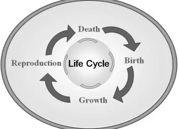
All living organisms have life cycle, either the commonest ants, butterflies, goldfish around us, or the uncommon Antarctic penguins, arctic bear; either ferocious beast or the meek of poultry. Although different organisms have different life-cycle lengths, but they all undergo the process from birth to death. With this process, even though an organism died, but the species will not perish. Through reproduction, species can continue from generation to generation. Four stages including birth, growth, reproduction, and death comprise the biologic life cycle [7]. Borrowing the biology life cycle theory, this paper presents a Lifecycle-based Swarm Optimization (LSO) technique. LSO algorithm is a population-based optimization method and employ six optimize operators according to features of life cycle theory.
In order to evaluate the performance of LSO, extensive studies based on a set of constrained benchmark functions has been carried out in this paper. Because many bio-inspired algorithms have been solved for real-world engineering optimization problems involving constraints and have obtained the better solution [8-11], such as structure optimization, mechanical design, VLSI design, economics, and allocation and location problems. So in this paper, LSO was also tested on practical vehicle route problems. For comparison purposes, we also implemented PSO and GA. Experimental results show that LSO has same superior search performance for constrained problems compared with other algorithms.
The rest of this paper is organized as follows. Section 2 introduces the life cycle theory. Section 3 describes the
Manuscript received October 8, 2010; revised November 1, 2010; accepted November 1, 2010.
proposed Lifecycle-based Swarm Optimization (LSO) technique. Sections 4 present the experimental results and discussion. In the next section, LSO was tested on the capacity vehicle routing problem and the experimental results were compared. The last section draws conclusions and gives directions of future work.
II. LIFE CYCLE THEORY
The biology evolution of nature follows the "cycle relay" pattern, which is a "life and death alternation" cycle process. When an original life ends, a new life will generate. This process repeated continuously made the endless life on earth, and biologic evolution become more and more perfecting. Life can continue just in this cycle process. Nature’s biology (from diatoms, algal group, lichens, and mosses, to the plants and animals), regardless of the species, should follow the "life and death alternation" cycle process [12]. In this pattern, the life cycles of different biology may seem very different at first glance. Some biologic life may be going through several decades, and some biologic life perhaps lasted only a very short time. In this pattern, the shape, the size and the reproduction mode of different organisms are also different, and life span is not the same. But they have similar life cycle characteristics. All life cycles shown in Fig. 1 are same in that they begin with birth and end with death. They are born; they need grow up; they can reproduce; they will death. "Life and death alternation" cycle process is not a simple repeat, but rather an incessant improvement, accumulation and perfection process, and is an optimal way of achieving ultimate goal of life.
Figure 1. Search strategy for foraging animal.
III. LIFECYCLE-BASED SWARM OPTIMIZATION
ALGORITHM
Population is the evolution unit and the specific existence form of life, so the initialization of population is represents the individuals’ birth stage [13].
Once an organism begins its life cycle, it immediately faces survival needs. For this purpose, most biology requires food, water, sunlight, minerals, and oxygen to survive and grow. They get these resources in many different ways. The behavior of get resources is called foraging. In the process of foraging, the choice of
foraging strategy is essential. A better foraging strategy makes forager get more resources in the shortest time, then forager would has enough nutrition to survive or breed the next generation. Conversely, if a forager selects the failing strategy continuously, and don’t gain nutrition resources, meanwhile its energy was also consumed, then it will be eliminated gradually according to the natural selection theory. Biologic foraging strategies are diverse. In LSO, we defined three foraging operators: chemotactic operator, assimilation operator and transposition operator. At the same time, we employed the reproduction and selection operator according to the reproduction and death stage of life cycle. In addition to, we also added mutation operator.
A. Chemotaxis Operator
Chaos exists widely in natural and social phenomena, its behavior are complex and similar to the random, and are a rather common phenomenon in nonlinear system [14]. Chaos motion should traversal all states which were not repeated in the way of its own "law" in a certain area. Chaos process seems confusion, in fact, it is not completely disorder, but exist subtle regularity inherent. Chaotic motion has ergodicity, randomness and regularity and the others features. Since 1970’s, a large number of biologic model simulation explained that the chaos is widespread exist in biologic systems.
Borrowing chaotic theory, chemotactic operator which was employed by the optimal individual of population will performs the chaos search strategy. The basic idea is introducing logistic map to optimization variables using a similar approach to carrier, and generate s set of chaotic variables, which can shown chaotic state [15,16]. Simultaneously, enlarge the traversal range of chaotic motion to the value range of the optimization variables. Finally, the better solution than current would found directly using chaos variable. The logistic map equation is given by equation (1):
)
1
(
1 i i
i
rx
x
x
+=
-
(1)where r (sometimes also denoted μ) is driving parameter, sometimes known as the "biotic potential", and is a positive constant between 0 and 4. Generally, r=4. xi represent the current chaos variable, and xi+1 represent the next time’s .
B. Assimilation Operator
) (
1
1 i p i
i X r X X
X+ = + - (2)
where r1
Î
Rn is a uniform random sequence in the range (0,1). XP is the best individual of the current population. Xi is the position of an individual who perform assimilation operator and Xi+1 is the next position of this individual.C. Transposition Operator
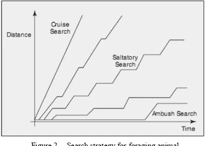
Biology has strong survival instincts, which would indicate organism foraging method. This is an individual behavior, which don’t reference to other individuals foraging information. Some animals are “cruise” or
“ambush” searchers [17]. For the cruise approach to searching, the some forager moves continuously through the environment constantly searching for prey. For the ambush approach to searching, some forager sits and waits for prey to cross into strike range. In fact, the search strategies of some forager are in between the cruise and ambush, that is “salutatory” search. Fig. 2 gives the illustration of these strategies. To find better living conditions, survival instincts lead animals to migrate to a better habitat. Some animals migrate only short distances. Some animals are continually migrating great distances.
Figure 2. Search strategy for foraging animal.
During each iteration, the rest individuals will perform transposition operator in a way of randomly migration within their own energy scope.
D × =( p i)
i X X
ub (3)
i
i ub
lb =- (4) j=r2(ubi-lbi)+lbi (5)
j
+ =
+ i
i X
X 1 (6)
where φ is the migration distance of Xi; r2
Î
Rn is a normal distributed random number with mean 0 and standard deviation 1; ubi and lbi is the search space boundary of the ith individual; Δ is the range of the global search space.C. Crossover Operator
Crossover operator means exchange of a pair of parent’s genes in accordance with a certain probability, and generates the new individual. In biologic life cycle, reproduction is an important feature. After individual mature, it will reproduction, whether sexual reproduction
or asexual reproduction. Reproduction makes the continuation of species.
In LSO, the crossover operator selects single-point crossover method. One crossover point is selected, string from beginning of individual to the crossover point is copied from one parent, and the rest is copied from the second parent.
D. Selection Operator
The reasons of biology death are varied. Some biology is illness or eaten by other predators or lack of nutrition resources for a long time and so on. But no matter what manner of biologic death, in general, those who survive is to adapt the living environment, which are eliminated are not suited to the biologic environment, which is Darwin's
“the survival of the fittest” theory. In this algorithm, when some offspring were produced, the size of the population will increase. Overmuch individual and the limited resources will inevitably result in the struggle for existence. Then the survival chance is bigger for some biology which has stronger vitality, whereas it is smaller for the biologic with weak vitality.
According to “the survival of the fittest” theory, and for ensuring a fixed population size, LSO take a certain method which can make some individuals were retained and others were eliminated. In this algorithm, the selection operator performs elitist selection strategy. A number of individuals with the best fitness values are chosen to pass to the next generation.
E. Mutation Operator
Mutations are changes in a genomic sequence. It is an accident in the development of the life, and is the result of adaptation to the environment. Mutations that change protein sequences are neutral or harmful for an organism, and also have a positive effect. When it is useful for a species or single organism, it would make them have more chances of survival, moreover it can continue in the future generations, and we can say that the evolution of species occurred. So mutation is important for the evolution, no mutation, and no evolution. A mutation may occur in any time in life cycle of an organism, and is common, random, low frequency and non-directional.
In LSO, the mutation operator performs dimension-mutation strategy. One dimension of an individual selected according to the probability will re-location in search space.
xij=rand(1)(ub-lb)+lb (7)
where ub and lb is the lower and upper boundary of search space. In the N-dimension search space, the xij is the position of the jth dimension of the ith individual; the value j is between in [1, N].
convergence to the optimal solution when the solution is closer to the optimal solution. It also can maintain population diversity for prevention premature convergence.
F. The Pseudo-code of LSO
Lifecycle-based Swarm Optimization is a population-based search technique, evaluation the fitness function, and establishes an iterative process through implementation six operators proposed above. Every population was composed by a certain number of individuals. In each iteration, firstly, an individual need choice foraging strategy and execute corresponding foraging operator based on own fitness value and foraging probability generated randomly, then followed by the mutation operation. The second stage is crossover
operation, followed by the mutation operation. The third stage is selection operation and followed by the mutation operation. Finally, generate the next population which can represent the new solutions. In the optimization process, the optimization operation is random, but the characteristics shown us are not entirely random search. It can effectively utilize the historical information to speculate the next solutions, which has the possible of closer to optimum. Such process was repeated from generation to generation, and finally converges to the individual which was the most adaptable to environments, obtained the optimal solution. The Pseudo-code of the algorithm is shown in TableI.
TABLE I.
PSEUDO CODE OF LIFECYCLE-BASED SWARM OPTIMIZATION ALGORITHM
Parameters Setting: Population size: S; dimensionality of search space: N; maximum iterations: Tmax; the lower and upper
limits of the global search space: Blo, Bup; driving parameter of chaos search: r=4; crossover
probability: Pc; mutation probability: Pm.
Born Stage: (1) Initialize the population with a normal distributed according to the U and Ө. (2) Compute the fitness values of all individuals.
Growth Stage: (1) The best individual of population executes the chemotaxis operator via the chaos searching using the equation (1).
(2) A number of individuals selected via will perform assimilation operator using the equation (2).
(3) The rest individuals would execute the transposition operator using the equations (3) to (6). (4) Execute dimension-mutation operation to Swarm using equation (7) based on the mutation probability.
Reproduction Stage: (1) Randomly select a pair of individuals to implement single-point crossover operation. All individuals generated by crossover operation comprised the offspring-population, which is called
SubSwarm.
(2) Execute dimension-mutation operation to SubSwarm based on the mutation probability. (3) Compute the fitness values of the SubSwarm, and perform elitist selection operation.
Death Stage: (1) Sort all individuals of Swarm and SubSwarm in order of ascending fitness.
(2) The S individuals with the lower fitness were selected and others with higher fitness die.
(3) Execute dimension-mutation operation to Swarm based on the mutation probability.
IV. EXPERIMENTS AND RESULTS
A. Parameters setting
To fully evaluate the performance of the LSO algorithm without a biased, we employed 13 benchmark functions [18]. These functions were tested widely in evolutionary computation domain to show the quality solution and the convergence rate. Problems g02, g03, g08 and g12 are maximization problems. They were transformed into minimization problems using –f(x). Problems g03, g05, g11 and g13 include one or several equality constraints. All of these equality constraints were converted into inequality constraints, f(x)-d£0 ,
δ=0.000001. For each problem, Table Ⅱ shows the following parameters:
l n: the number of variables. l f : the type of objective function.
l ρ: the ratio between the feasible region and the whole search space.
l LI: the number of linear inequalities. l NI: the number of nonlinear inequalities. l NE: the number of nonlinear equations.
of function g01, g02, g04, g06, g07, and g09 lies on the boundaries of the feasible region.
B. Parameters setting
We compared the optimization performance of LSO with the standard PSO. Experimental results are summarized in Table III. Each algorithm was tested with all numerical benchmarks and each experiment was repeated 30 times. In every run, the max iterations Tmax =3000. With the purpose of making the comparison fairly, the initialization populations for all the considered algorithms were generated using the same population. The same population size S=50.
In LSO, the probability using for decision the individual’s foraging strategy Pf=0.1; the number of chaos variables Sc=100; crossover probability Pc=0.7; mutation probability Pm=0.02; the selection operation is roulette wheel method. The PSO algorithm we used in this paper is the standard algorithm. In PSO, the acceleration factors c1=1, and c2=1.49; and a decaying inertia weight w starting at 0.9 and ending at 0.4 was used. For every problem, the most common approach adopted to deal with constrained search spaces is the use of penalty functions [19]. In this paper, the penalty coefficient is a great value.
TABLE II.
CHARACTERISTICS OF THE TEST FUNCTIONS
TF n Type of f ρ LI NI NE a
g01 13 quadratic 0.000235% 9 0 0 6
g02 20 nonlinear 99.996503% 1 1 0 1
g03 10 polynomial 0.000000% 0 0 1 1
g04 5 quadratic 26.962511% 0 6 0 2
g05 4 cubic 0.000000% 2 0 3 3
g06 2 cubic 0.006679% 0 2 0 2
g07 10 quadratic 0.000103% 3 5 0 2
g08 2 nonlinear 0.859082% 0 2 0 0
g09 7 polynomial 0.524450% 0 4 0 2
g10 8 linear 0.000522% 3 3 0 3
g11 2 quadratic 0.000000% 0 0 1 1
g12 3 quadratic 4.775265% 0 1 0 0
g13 5 nonlinear 0.000000% 0 0 3 3
TABLE III. BEST VALUES OF LSO AND PSO
Problem Optimal value LSO PSO
g01 -15 -14.822 -15
g02 0.803619 0.79982 0.77738
g03 1 0.608 0
g04 -30665.539 -30643 -30665
g05 5126.4981 5128.6 5131.1
g06 -6961.81388 -6961.8 -6961.8
g07 24.3062091 25.849 24.885
g08 0.095825 0.095825 0.095825
g09 680.630057 680.63 680.63
g10 7049.25 7085.9 7172.3
g11 0.75 0.75009 1
g12 1 0.48473 0.48473
g13 0.0539498 0.045187 0.031081
TABLE IV.
WORST VALUES OF LSO AND PSO
Problem Optimal
value LSO PSO
g01 -15 -14.594 -9
g02 0.803619 0.73567 0.27602
g03 1 0.12609 0
g04 -30665.539 -30503 -30186
g05 5126.4981 --- ---
g06 -6961.81388 -6960.6 ---
g07 24.3062091 43.869 1638
g08 0.095825 0.095825 0.095825
g09 680.630057 681.76 680.72
g10 7049.25 8726.2 ---
g11 0.75 0.99877 1
g12 1 --- ---
g13 0.0539498 --- ---
(---: infeasible solution)
TABLE V.
MEAN VALUES OF LSO AND PSO
Problem Optimal value LSO PSO
g01 -15 -14. 706 -11.067
g02 0.803619 0. 77112 0.52251
g03 1 0.10723 0
g04 -30665.539 -30571 -30656
g05 5126.4981 5467 13461
g06 -6961.81388 -6961. 5 -4096.5
g07 24.3062091 33. 203 205. 47
g08 0.095825 0. 095825 0. 095825
g09 680.630057 680.87 680.66
g10 7049.25 7721. 6 41034
g11 0.75 0. 89687 1 g12 1 40000 6.4e+005
g13 0.0539498 8e+005 7.6e+005
TABLE VI.
STANDARD DEVIATION VALUES OF LSO AND PSO
g01 0.066098 2.0998 g02 0.019706 0.11555
g03 0.17369 0
g04 76.481 67.795
g05 3248. 2 12437 g06 0.26245 15694 g07 4.7188 310.21
g08 5.16E-17 2.49E-17
g09 0.2187 0.023907
g10 475.34 1.18E+05
g11 0.090638 0
g12 1.98e+05 4.85e+05
g13 4.041e+005 4.314e+005
V. DISCUSSION OF RESULTS
This paper compared LSO against PSO. The best results obtained in 30 runs by each approach are shown in Table III. The worst results are presented in Table IV, the mean values provided are compared in Table V and the standard deviations are listed in Table VI. Moreover, the optimal solutions known so far are also presented in Table III, Table IV and Table V.
In Table III, an objective function value with bold typeface indicates that the corresponding solution is exactly equal to the best known solution. LSO can find the exact global optimum in four functions (g04, g06, g08, g09 and g11) and close to the global optimum in eight functions (g01, g02, g03, g04, g05, g07, g12 and g13). PSO find the exact global optimum in five functions (g01, g04, g06, g08 and g9) and close to the global optimum in seven functions (g02, g03, g05, g07, g11, g12 and g13). Judging from the best solutions obtained by them, the performance of PSO is better than LSO.
From table IV we can see LSO performs better than the PSO. Firstly, LSO can’t seek the feasible solutions in 30 runs on three functions (g05, g12 and g13) and PSO can’t seek it on 5 functions (g5, g6, g10, g12 and g13). Moreover it is worth noticing that all of the “worst” result obtained by LSO is even also the approximately global optimum solution in most of the problems. Both LSO and PSO can find the close to the global optimum solution in function g01, g02, g03, g04, g08, g09 and g011. Especially in functions g06 and g10, the solutions found by LSO are feasible and also near to the global optimum, but solutions found by PSO are infeasible.
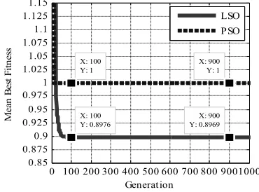
Table V and VI presents the mean solution and standard deviation in 30 independent runs. In these two tables, the value with bold typeface all indicates the better solution and lower standard deviation of two methods. With the exception of g04, g09 and g13, in all the other problems LSO reached the exact or close to global optimum and better than PSO. On most of problems, LSO presented a lower standard deviation. Fig.3~ Fig.7 are the convergence curve of LSO and PSO in some functions.
The values of each point in curves are the mean best values in 30 independent runs.
For function g01 and g11 which is shown in Fig. 3 and Fig. 4, in less than 100 iterations, both LSO and PSO have the fast convergence rate. Convergence curves of them decline rapidly and converge to local optimum solution, which was obtained by LSO and is better than PSO’s. From 100 iterations to end, the curve of PSO is still a straight line. It can’t find a better solution and deeply fall into the local optimum solution. However, LSO is different due to its ability of diversity, which can make LSO jump out of local optimal solution. For function g01 shown in Fig. 3, from 100th to 1000th iterations, the curve of LSO can continues to decline even though the speed is slow. In the end, LSO obtain the approximately global optimum solution. For function g11 shown in Fig 4, at the 100th iteration, both LSO and PSO have found near to the global optimal solutions 0.8976 and 1, respectively. The value obtained by LSO is better than PSO’s, and this situation continued until the end.
0 100 200 300 400 500 600 700 800 900 1000 -16
-15 -14 -13 -12 -11 -10 -9 -8 -7 -6
X: 100 Y: -12.66 X: 100 Y: -10.5
X: 962 Y: -14.55
Generation
M
ea
n
B
es
t F
itn
es
s
X: 962 Y: -10.67
LSO PSO
Figure 3. Details of convergence curve in the first 1000 iterations on function g01.
0 100 200 300 400 500 600 700 800 9001000 0.85
0.875 0.9 0.925 0.95 0.975 1 1.025 1.05 1.075 1.1 1.125 1.15
X: 100 Y: 0.8976 X: 100 Y: 1
X: 900 Y: 1
X: 900 Y: 0.8969
Generation
M
ea
n
B
es
t F
itn
es
s
LSO PSO
Figure 4. Details of convergence curve in the first 1000 iterations on function g11.
converge to a local solution. With the increasing in the number of iterations, solution found by LSO is gradually close to the global optimum. Compared with LSO, at the beginning of iteration, PSO has the very slow convergence speed and converge to a local solution until about the 400th iterations. At the end of iterations, PSO still don’t find the exact or approximately optimal solution. Moreover, the bigger standard deviation demonstrates that the PSO has a strong instability.
0 100 200 300 400 500 600 700 800 9001000 -1 -0.75 -0.5 -0.25 0 0.25 0.5 0.75
1x 10
4
X: 100
Y: -5957 X: 988 Y: -6940 X: 436 Y: -1199 Generation M ea n B es t F itn es s X: 988 Y: -1231 LSO PSO
Figure 5. Details of convergence curve in the first 1000 iterations on function g06.
For function g06, the global optimal solution is -6961.8. At the 100th iterations, the solution -5957 found by LSO is begun to approach it. However, at the 436th iterations, the solution -1199 found by PSO is still very far away from it. At about 988th iteration, the solution -6940 found by LSO is better than obtained in the early and is close to optimal solution. But the value -1231 found by PSO is still a worst solution.
0 250 500 750 1000 1250 1500
0 100 200 300 400 500 600 700 800 900 1000 X: 1400 Y: 32.68 X: 100 Y: 50.72 X: 1400 Y: 442.4 X: 401 Y: 470.7 Generation M ea n B es t F itn es s LSO PSO
Figure 6. Details of convergence curve in the first 1500 iterations on function g07.
Similarly, for function g07, the process of seeking optimum and the quality of the final solution of LSO and PSO is the same with function g06. Even if the true optimal solutions not found by these two algorithms, we still can observe that LSO also obtained a better “worst”
result than PSO. On functions g12, LSO has sought the feasible solution but PSO hasn’t.
A remarkable example is g05, g10 and g12, where LSO and PSO were not able to reach the global optimum and showed a considerably high variability of results from run to run. This may be due to the fact that function
g10 has a large search spaces (based on the intervals of the decision variables) with a very small feasible region; function g05 have small feasible regions and its type of combined constrained is cubic and function g12 has even disjoint feasible regions. On functions g05 and g10, LSO has sought the close to optimal solutions but PSO can’t. As described in Fig. 7, before the 1785th iteration, LSO converge rapidly and find a close to optimal solution 5561, but the value 1.49e+4 found by PSO is far away from the optimum. From the 1785th iteration to end, the solution of PSO still can’t obtain great improve.
0 500 1000 1500 2000 2500 3000
0.05 1.05 2.05 3.05 4.05
5x 10
4 X: 1785 Y: 5561 Generation M ea n B es t F itn es s X: 1785 Y: 1.49e+004 LSO PSO
Figure 7. Details of convergence curve on function g05.
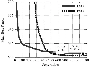
Only for function g04, g09 and g13, PSO perform better than LSO. Function g04 is a moderately constrained problems; g09 is a highly constrained problems with moderated dimensionality. For these two functions, LSO and PSO all find the close to optimal solution, which was found by LSO slightly worst than PSO’s. We can see from Fig. 8, on function g09, LSO has the same fast convergence speed as PSO in the early evolution, but gradually the convergence speed of LSO is slower than PSO, and obtained a relative poor value in the end. Function g13 has small feasible regions, and its type of combined constrained is nonlinear. On this function, the best mean values of two methods are all very worst.
0 100 200 300 400 500 600 700 800 900 1000 680 685 690 695 700 X: 549 Y: 681.1 Generation M ea n B es t F itn es s X: 948 Y: 681.4 LSO PSO
Figure 8. Details of convergence curve in the first 1000 iterations on function g09.
VI. LSO IN SOLVING VEHICLE ROUTING PROBLEM
as compared with other existing methodologies, the Vehicle Routing Problem (VRP) benchmark instance was selected as the testing case. VRP is a very complex combinatorial optimization problem and the commonest problem in logistics distribution system. Its purpose is to design the least costly (distance, time) routes for a fleet of capacities vehicles to serve geographically scattered customers. Because complexity of the actual problem, so there are many restrictions in VRP such as the capacity for each vehicle, total traveling distance allowed for each vehicle, time window to visit the specific customers, and so forth. VRP has been proved to be an NP-complete problem [20, 21].
A. Problem despcrition of VRP
The VRP is described as follows: The problem with one center storehouse and some customers is considered. Some vehicles are available to carry the cargo for all the customers. The main objective function is to minimize the transport cost. Generally the transport cost is simplified as the routing length. Assume that the depot is node 0(i=0), and L(i=1,2,…,L) customers are to be served by K(k=1,2,…,K) vehicles, the demand of customer i is gi, the capacity of vehicle q, the distance of traveling from customer i to customer j is cij. Then the objective function is shown as below:
åå å
= = = Kk L
i L
j
c
ijx
ijk 1 0 0 mizemin (8)
Subject to:
å
iL=1giyki£q, "k (9)
å
Kk=1yki =1, i=1,L,L; "k (10)
å
iL=0xijk =ykj,i=1,L,L; "k (11) L x y i L kj ijk = ki = "
å
=0 , 1,L, ; (12) where xijk is a binary variable indicating whether vehicle k arrives at node j from node i, if vehicle k arrives at node j from node i, then xijk=1, otherwise, xijk =0. yki is a binary variable indicating whether the node i is served by vehicle k, if the node i is served by vehicle k, then yki =1, otherwise, yki=0. The objective function in (8) aims to minimize the total distance. Constraint set (9) regulates that the load of each vehicle should not exceed its capacity. Constraint set (10) represents each customer demand must be satisfied and only fulfilled by one vehicle. Constraint sets (11) and (12) ensure that there has only one vehicle which arrival and departure from a customer.B. Experiment and resuslts
The computation data was cited from [22]. It was shown as follows: a distribution center delivers products to eight customers by two vehicles; each customer’s demand and the distance matrix were listed in Table IV, in which the value 0 indicates the distribution center. The load capacity and the speed of vehicles are 8t and 50km/h, respectively. The demand of this problem is arrange the
vehicle requested route reasonable, and make the total costs minimum, which is the shortest transportation distance.
TABLE VII.
CUSTOMER’S DISTANCE AND DEMAND
C 0 1 2 3 4 5 6 7 8
0 0 4 6 7.5 9 20 10 16 8
1 4 0 6.5 4 10 5 7.5 11 10
2 6 6.5 0 7.5 10 10 7.5 7.5 7.5
3 7.5 4 7·5 0 10 5 9 9 15
4 9 10 10 10 0 10 7.5 7.5 10
5 20 5 10 5 10 0 7 9 7.5
6 10 7.5 7.5 9 7.5 7 0 7 10
7 16 11 7.5 9 7.5 9 7 0 10
8 8 10 7.5 15 10 7.5 10 10 0
Demand 1 2 1 2 1 4 2 2
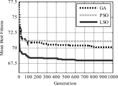
For this instance, this paper adopts the real number encoding [23]. In this paper, the LSO was compared with two well-known algorithms: PSO and GA. In experiment, the individual numbers, S=60; the max iterations Tmax =1000, each experiment was repeated 30 times. The rest parameters setting of LSO and PSO are same as the section IV. The crossover probability and mutation
probability of GA is 0.7 and 0.5, respectively. Table VIII shows the comparison results of three algorithms. In this table, an objective function value with bold typeface indicates that the corresponding solution is exactly equal to the best known solution. The “Worst” and the “Best”
represents the maximum and the minimize value obtained by these methods, respectively. The success ration means the number of seeking the exactly optimal solution in 30 runs.
TABLE VIII.
THE EXPERIMENTAL RESULTS OF THREE ALGORITHMS
LSO PSO GA
Worst 69 74.5 74
Best 67.5 67.5 67.5
Mean Best 67.95 71.1 70.117
Std 0.6991 1.6421 1.4953
Success ratio 20 11 9
best-known solutions. But the contrary results were obtained by PSO and GA, there are a few successes run in 30 runs. In term of computational effort as shown in Fig. 9, LSO is faster than other algorithms.
0 100 200 300 400 500 600 700 800 900 1000 67.5
70 72.5 75 77.5
Generation
M
ea
n
B
es
t F
itn
es
s
GA PSO LSO
Figure 9. Convergence curve of LSO, PSO and GA.
VII. CONCLUSIONS
Based on biological life cycle theory, this paper proposed a Lifecycle-based Swarm Optimization algorithm. In this algorithm, six operators were employed: chemotactic, assimilation, transposition, crossover, selection and mutation. An individual in the population gradually grow though performing either chemotactic operator, or assimilation operator or transposition operator. Population generates offspring via crossover operation. Some individuals will die using selection operation. Additionally, biological mutation may occur at any time, this method employ mutation operator. The approach was tested using 13 widely used benchmark problems, which include various constrained problems, and a small-scale vehicle routing problem. On 13 benchmark functions, the results obtained showed a very substantial potential of LSO based on quality of results. LSO can seek the feasible optima solution of almost all test cases, but PSO can’t, and on some problems, LSO’s performance remarkably outperforms other algorithms. Meanwhile, the standard deviations also reveal the strong robustness of LSO. Since the performance of LSO on test function g05, g012 and g13 is not satisfied, a more profound study in improving LSO though tuning parameters or other method is absolutely necessary in future work. Another direction of future work is to apply this method to the large-scale vehicle routing problem or other areas.
ACKNOWLEDGMENT
This project is supported by the National 863 plans projects of China (Grant No. 2008AA04A105), and the Doctoral start fund of Liaoning province of China (Grant No. 09L3170301).
REFERENCES
[1] Y. Yuan, Z. He and M. Chen, “Virtual mimo-based cross-layer design for wireless sensor networks”, IEEE
Transactions on Vehicular Technology, vol. 55, no. 3, pp. 856-864, May 2006.
[2] S. C. M. Cohen and L. N. de Castro, “Data clustering with particle swarms”, In the Proceedings of IEEE Congress on Evolutionary Computation, Vancouver BC, pp.1792-1798, 2006.
[3] A. V. Donati, R. Montemanni and N. Casagrande et al.
“Time dependent vehicle routing problem with a multi ant colony system”, European Journal of Operational Research, vol.185, no.3, pp.1174–1191, March 2008. [4] F. Campelo, F. G. Guimaraes and H. Igarashi, “A clonal
selection algorithm for optimization in electromagnetics”, IEEE Transactions on Magnetics, vol. 41, no. 5, pp.1736-1739, May 2005.
[5] C. F. Juang, “A hybrid of genetic algorithm and particle swarm optimization for recurrent network design”, IEEE Transactions on Systems Man and Cybernetics Part B Cybernetics, vol. 34, no. 2, pp.997-1006, April 2004. [6] J. J. Davis, Training product unit neural networks with
genetic algorithms”, IEEE Expert: Intelligent Systems and Their Applications, vol. 8, no. 5, pp.26-33, October 1993. [7] D. A. Roff. The evolution of life histories: theory and
analysis. Chapman and Hall, New York, 1992.
[8] S. Koziel and Z. Michalewicz, “Evolutionary algorithms, homomorphous mappings, and constrained parameter optimization”, Evolutionary Computation, vol. 7, pp. 19-44, Spring 1999.
[9] K. Deb, “An efficient constraint handling method for genetic algorithms”, Computer methods in applied mechanics and engineering, vol. 186, pp.311-338, June 2000.
[10]C. A. C Coello, “Constraint-handling using an evolutionary multiobjective optimization technique”, Civil engineering and environmental systems, vol. 17, pp. 319-346, October 2000.
[11]Z. Michalewiz and M. Schoenauer, “Evolutionary algorithms for constrained parameter optimization problems”, Evolutionary Computation, vol. 4, pp. 1-32, spring 1996.
[12]S. C. Stearns. The evolution of life histories. Oxford University Press, UK, 1992.
[13]J. H. Vandermeer and D. E. Goldberg. Population ecology: first principles. Princeton University Press, Woodstock, 2003.
[14]S. M. Berman. Mathematical statistics: an introduction based on the normal distribution. PA: Intext Educational Publishers, Scranton, 1971.
[15]E. N. Lorenz, “Deterministic non-periodic flow”, Journal of the Atmospheric Sciences, vol. 20, pp.130–141, 1963. [16]P. F. Verhulst, “Recherches mathématiques sur la loi
d'accroissement de la population”, Nouv. mém. de l'Academie Royale des Sci. et Belles-Lettres de Bruxelles, vol. 18, pp.1-41, 1845.
[17]K. M. Passino. Biomimicry for optimization, control, and automation. Springer-Verlag, London, UK, 2005. [18]T. P. Runarsson and X. Yao, “Stochastic ranking for
constrained evolutionary optimization,”IEEE Transactions Evolutionary Computation, vol. 4, pp. 284–294, September 2000.
[19]J. T. Richardson, M. R. Palmer and G. Liepins, et.al, ,
“Some guidelines for genetic algorithms with penalty functions,” In the Proceedings of the 3rd International Conference on Genetic Algorithms, SanMateo, CA, pp. 191–197, June 1989.
[21]M. Haimovich, R. Kan and L. Stougie, Analysis of heuristics for vehicle routing problems. In Vehicle routing: methods and studies, North-Holland, 1988.
[22]L. P. Zhang and Y. T. Cai, “Improved Genetic Algorithm for Vehicle Routing Problem”, Systems Engineering-Theory & Practice, vol. 22, no. 8, pp. 79-84, August 2002. [23]J. Li, B. L. Xie and Y. H. Guo, “Genetic algorithm for vehicle scheduling problem with non-full load”, System Engineering Theory Methodology Applications, vol. 20, no. 3, pp. 235-239, September 2000.
Hai Shen was born in China in 1976. She has received the B.Sc. and M. Eng. Degrees in computer applications technology,Shenyang University of Technology, Shenyang, China, in 1998 and 2005, respectively. She is currently working toward the Ph.D. degree with the Shenyang Institute of Automation, Chinese Academy of Sciences, China. Now, she is an Associate Professor with the College of Physics Science and Technology, Shenyang Normal University, China. Her main research interests are in advanced computational intelligence with a focus on: nature inspired hybrid intelligent systems, swarm intelligence, evolutionary computation, distributed artificial intelligence, multi-agent systems and other heuristics swarm intelligence.
Yunlong Zhu is the director of the Key Lab. of Advanced Manufacturing Technology, Shenyang Institute of Automation of the Chinese Academy of Sciences. He received his Ph.D. in 2005 from the Chinese Academy of Sciences, China. He has research interests in various aspects of Enterprise Information Management but he has ongoing interests in Artifical Intelligence, Machine Learning, and related areas. Prof Zhu’s research has led to a dozen professional a publication in these areas includes the biography here.