ISSN (e): 2250-3021, ISSN (p): 2278-8719
Vol. 08, Issue 8 (August. 2018), ||V (I) || 58-65
A Comparative Analysis Of Clustering Based Brain Tumor
Segmentation Techniques
Dr. Ardhendu Mandal,
Kanishka Sarkar,
Tanmoy Kanti Halder
Dept. Of Comp Sc And Application, University Of North Bengal, Darjeeling Corresponding Author:Dr. Ardhendu Mandal
Abstract:
Image segmentation of human brain is commonly used for clear-cut partitioning of gray and white matter, cerebral spinal fluid and skull in the image. Several image segmentation strategies have been proposed from the early stages of image processing. Clustering is one of the most popular among them. In this work k-mean, Fuzzy c mean and Genetic algorithm based clustering techniques has been studied and comparative analysis has been done in terms of mean and variance of segmented tumor, and inter and intra cluster distance of the centers for individual algorithm. The accuracy of each method is also compared with the ground truth image. The implemented clustering methods are further compared based on some segmentation metric. Here the BRATS-12 dataset is used for testing the algorithms, which consists 27 high grade tumor and 15 low grade tumor MRI images. Each MRI image is given with four different modalities such as T1, T2, FLAIR and T1+C. The database also consist four ground truth segmented images for each image. The ground truth images are prepared by the four different observers.Index Terms
: brain tumor, clustering, fuzzy c-mean, genetic algorithm, k mean, segmentation.--- --- Date of Submission: 20-07-2018 Date of acceptance: 04-08-2018 --- ---
I.
INTRODUCTION
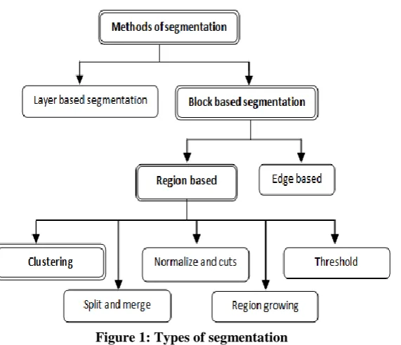
mage segmentation is the process of dividing an image into specific sections based on different levels of certain parameters to clearly identify objects from the original image. Brain image segmentation is very critical and sensitive as it is related with the human life. Hence, it further requires minimum segmentation error. There can be two measure types of image segmentation. One is block based and another is layer based. The block based segmentation can be broadly classified into the following two categories.
This paragraph of the first footnote will contain the date on which you submitted your paper for review. It will also contain support information, including sponsor and financial support acknowledgment. For example, “This work was supported in part by the U.S. Department of Commerce under Grant BS123456.”
The next few paragraphs should contain the authors‟ current affiliations, including current address and e-mail. For example, F. A. Author is with the National Institute of Standards and Technology, Boulder, CO 80305 USA (e-mail: author@ boulder.nist.gov).
S. B. Author, Jr., was with Rice University, Houston, TX 77005 USA. He is now with the Department of Physics, Colorado State University, Fort Collins, CO 80523 USA (e-mail: [email protected]).
T. C. Author is with the Electrical Engineering Department, University of Colorado, Boulder, CO 80309 USA, on leave from the National Research Institute for Metals, Tsukuba, Japan (e-mail: [email protected]).
i) Region Based
ii) Edge Base or Boundary Base
The region based segmentation further classified in the following categories [1]. i) Clustering
Figure 1: Types of segmentation
Clustering is widely used for segmenting medical images. Clustering algorithms are used to partition a dataset into a certain number of group, subsets or categories, where the data members of each group are similar while the data members from different group are not [2]. Different researchers adopted different clustering techniques for medical image segmentation. Among them k-mean, fuzzy c-mean and genetic algorithm based clustering techniques are most popular.
K-mean has been chosen as clustering approach by several researchers because of its simplicity. In k-means, there are k number of clusters (where, k≥ 2) and each data item belongs to any one of those clusters with the minimum mean (of?). Ming-Ni Wu, Chia-Chen Lin and Chin-Chen Chang [3] proposed a color based k mean clustering segmentation technique for brain tumor detection. In some later work color converted k-mean clustering segmentation technique [4] is proposed by Li-Hong Juang and Ming-Ni Wu. J. Vijay and J. Subhashini also used k-mean clustering algorithm [5].
In k-mean fuzzy clustering, whether a data item will belong to a cluster or not shall depend together on the probability that the data item is to be a member of a cluster and on the fuzziness coefficient in the membership function. Thus, k-mean fuzzy clustering allows a data item to be a member of more than one cluster. For this reason k-mean fuzzy clustering remains a good choice for image segmentation.
Although genetic algorithm is basically inspired from the biological sciences, but Mr. Ujjwal maulick and Sanghamitra bandyopadhyay [13] has shown in their work that it can be effectively used as a clustering technique. Further, G Rajesh Chandra and Kolasani Ramchand H Rao used genetic algorithm based clustering [14] for brain tumor segmentation with an effective success rate 97%.
N. Nandha Gopal and M. Karnan used fuzzy k- mean along with genetic algorithm and particle swam optimization techniques [7]. On the other hand support vector machine classifier is also associated with fuzzy c means by Parveen and Amritpal Singh [9]. Further, M. Shasidhar, V. Sudheer Raja and B. Vijay Kumar modified the fuzzy c mean algorithm to minimize convergence time [10] by using a comprehensive feature vector space to do the segmentation. A. Rajendran and R. Dhanasekaran also used region based fuzzy clustering in their work [11]. In some other work [8] region growing method is also integrated with the fuzzy clustering. Even not only brain, fuzzy c mean is also used to segment lung tumor [12]. Again, Garima Singh and M.A. Ansari use Naive Bayes classifier and SVM to determine whether there is tumor or not [6].
II.
METHODS
A. k-mean Algorithm1. Take input image of size r*c and convert it into grayscale 2. Set number of required cluster (k)
3. Partition the intensity range of input image equally into number of required clusters(k) by identifying the cluster having minimum distance for each pixel of input image and include the pixel intensity into its corresponding cluster set
4. Update the partition value of each cluster i.e. Cluster[k] as mean of its cluster set
Cluster k = Min intensity +Max intensity – Min intensity
Total no . of clusters ∗ k (1)
6. Distinguish pixels of each cluster set with distinct intensity in image matrix. 7.
B. fuzzy c-mean Algorithm
1. Take input image of size [r, c] and convert it into grayscale. 2. Convert image into a 1D array of size [1, r*c] i.e. ARR[r*c]. 3. Set value for fuzziness i.e. m and number of cluster required i.e. nc.
4. Choose initial centroid for each cluster randomly i.e. Centroid[j]=random, for j=1 to nc.
5. Compute membership function i.e. MFN for each pixel in ARR[i] against each centroid in Centroid[j] as:
𝑀𝐹𝑁𝑖𝑗 = 1 ÷
𝑑𝑖𝑗 𝑑𝑖𝑘
2 𝑚 −1
𝑛𝑐
𝑘=1
(2)
Where dij= Distance between ARR[i] and Centroid[j] 6. Now Calculate new centroid as:
Centroid[j] = (𝑀𝐹𝑁𝑗𝑖)𝑚 ∗ 𝐴𝑅𝑅 [𝑖]
𝑐∗𝑟 𝑖=1
𝑀𝐹𝑁𝑗𝑖
𝑐∗𝑟 𝑖=1
(3)
7. If difference between previous and current centroid is greater than .001 then go to step 5.
8. For each cluster identify the cluster with minimum MFN and distinguishcorresponding pixel in ARR[r*c] with distinct intensity.
9. Revert the updated 1D array i.e. ARR[r*c] to 2D image matrix.
C. Genetic Algorithm (GA) based Clustering
GA based clustering offers an effective technique to find the appropriate cluster centers. A new population with a better fitness value is generated in each iteration. In other words it actually optimizes the similarity metric of the cluster. Here in this case the chromosomes are consisting of four floating point value representing the cluster centres. The population is initialized with four chromosomes. This technique randomly selects two chromosomes for crossover and mutation to generate a new chromosome and it is repeated for 4 times. The termination criterion is set to 100th iteration.
Chromosome representation
Here the chromosome string consist of four randomly generated number in the range between 0 and maximum intensity value of the input image.
Example:
Chromosome_1=[32.3816 120.809 207.7545 230.9769] Population initialization
The population consists of 4 chromosomes. There can be any number of chromosomes in the population, but for simplicity here only 4 chromosomes is taken.
Fitness computation
Fitness computation is done into two phase. In the first phase the clustering is performed by assigning each point to the appropriate cluster with centre zj.
𝑥𝑖 ∈ 𝑐𝑗
Then new cluster centres are determined by computing the mean of each corresponding cluster. In the second phase the actual computation of fitness function is performed as follows.
𝜇 = 𝜇𝑖
𝑘
𝑖=1
𝜇𝑖 = |𝑥𝑗− 𝑧𝑖| 𝑥𝑗∈𝑐𝑖
And the fitness function is defined as 𝑓 = 1/𝜇 that means for minimum distance (𝜇) it maximizes𝑓.
i. Selection
A range of value is assigned to each chromosome for selection based on their fitness value such that to make the sum of total range is equal to 1. In the next step an random number is generated and the corresponding chromosome is selected in which it lies.
ii. Crossover
iii. Mutation
In mutation process any one of the values in the chromosome is modified. It is done by determining the mutation point in the similar way by generating a number between 1 to 4 and a value x is added to the corresponding value in the chromosome. Where x varies from -10 to +10.
Termination criteria
Genetic Algorithm is a NP Complete problem. It always leads to better solution, but the best solution cannot be achieved in real time. Instead it is suitable to optimize the solution. Here the solution is optimized up to 100th iteration.
III.
RESULT
AND
DISCUSSION
All three above discussed clustering algorithms has been implemented in MATLAB 13. In this section the result of these algorithms are discussed with comparative analysis. The comparison is done based on the clustering metric and segmentation metric. In case of clustering metric, the comparison has been shown in terms of inter-cluster distance and intra-cluster distance, where inter-cluster distance measures how pixels are co-related within a cluster and intra-cluster distance measures how two or more clusters are co-related. It is always desirable to minimize the inter-cluster distance and maximize the intra-cluster distance. Equation (4) is used to compute intra-cluster distance as follows.
|𝑐𝑖− 𝑐𝑗 | (4) 𝑘
𝑖,𝑗 =1
Where 𝑖 ≠ 𝑗, ci and cj represents centroid of ith and jth cluster respectively and k is the number of cluster.
And for the kth cluster the inter-cluster distance computed as below.
|𝑐𝑘− 𝑥𝑖| 𝑛
𝑖=1
𝑛 (5)
Where 𝑥𝑖 ∈ 𝑐𝑘 and n is the total number of elements in cluster k.
On the other hand for segmentation metric, two different measure approaches has been applied. Firstly, the comparison is given in terms of mean(µ) and variance(σ2) of segmented tumor. The following equations are used to evaluate mean and variance.
µ= 𝑥𝑖
𝑛 (6)
σ2= (𝑥𝑖−µ)2
𝑛 (7)
Where 𝑥𝑖 ∈ 𝑐4 and „n‟ is the total number of intensities in cluster 4.
Table 1 clustering metric results of fuzzy c mean Cluster wise Inter cluster Distance Intra-cluster Distance Mean of segmented Area Varience of segmented Area
6,6,1,23 78.31226985 173.9043478 93.55942029 8,9,5,1 41.80807445 92.5908142 29.03038738 8,6,1,7 51.20115052 114.0051037 44.46251994 15,2,11,8 64.25361816 137.9640206 80.82467162 20,8,2,7 68.65604344 154.1303879 72.24946121
Table 2: clustering metric results of k mean Cluster wise Inter cluster Distance Intra-cluster Distance Mean of segmented Area Varience of segmented Area
3,9,14,18, 77.45287505 168.9377818 73.13165014 2,11,8,15, 64.22515616 137.3928571 82.66573661 1,7,6,8, 51.02930397 114.0051037 44.46251994 1,6,6,23, 76.15119969 172.7380282 93.6 2,8,6,20, 61.41783622 137.3942857 61.33142857
3,11,14,7, 98.2147 179.5409 63.118 4,11,13,8, 78.1063 151.7681 40.733 1,7,7,5, 54.3939 106.1115 83.279 1,7,10,17, 83.0902 146.9651 52.144 2,9,12,12, 85.3040 153.2177 161.69
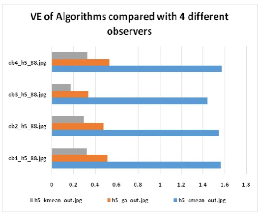
Secondly, the comparison shows the Volume Error(VE), Coefficient of Similarity(COS), Spatial Overlap(SO), Under Segmentation Rate(USR) and Over Segmentation Rate(OSR) of the segmented output image of each algorithm with respect of four different observers of the BRATS dataset. The equations for these metric are given below.
Volume Error, 𝑉𝐸 =2(𝑆−𝐺𝑆)
(𝑆+𝐺𝑆) (8)
Coefficient of Similarity, 𝐶𝑂𝑆 = 1 +(𝐺𝑆∩𝑆)
𝐺𝑆 (9)
Spatial Overlap, 𝑆𝑂 =2(𝐺𝑆∩𝑆)
(𝑆∪𝐺𝑆) (10)
Under Segmentation Rate, 𝑈𝑆𝑅 = |𝐺𝑆 − 𝑆 ∩ 𝐺𝑆 | (11) Over Segmentation Rate, 𝑂𝑆𝑅 = |𝑆 − 𝑆 ∩ 𝐺𝑆 | (12)
As per above discussion the following results are obtained.
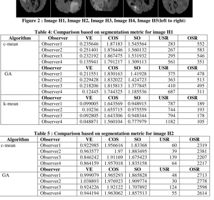
Figure 2 : Image H1, Image H2, Image H3, Image H4, Image H5(left to right)
Table 4: Comparison based on segmentation metric for image H1
Algorithm Observer VE COS SO USR OSR
c-mean Observer1 0.235646 1.87183 1.545564 283 552 Observer2 0.251401 1.876446 1.560132 267 583 Observer3 0.232192 1.867475 1.531932 295 546 Observer4 0.135941 1.791217 1.309113 561 351
Observer VE COS SO USR OSR
GA Observer1 0.211551 1.830163 1.41928 375 478 Observer2 0.229428 1.832022 1.424723 363 513 Observer3 0.218206 1.815813 1.377845 410 495 Observer4 0.12445 1.744325 1.185536 687 311
Observer VE COS SO USR OSR
k-mean Observer1 0.099005 1.643569 0.948915 787 189 Observer2 0.10236 1.655715 0.975559 744 193 Observer3 0.092805 1.643306 0.948344 794 178 Observer4 0.048871 1.560104 0.777979 1182 105
Table 5 : Comparison based on segmentation metric for image H2
Algorithm Observer VE COS SO USR OSR
c-mean Observer1 0.922985 1.956616 1.83368 60 2319 Observer2 0.963577 1.97 1.883495 39 2381 Observer3 0.846242 1.91169 1.675423 139 2207 Observer4 0.864159 1.957018 1.835158 64 2217
Observer VE COS SO USR OSR
Observer VE COS SO USR OSR
k-mean Observer1 0.955786 1.963847 1.860433 50 2486 Observer2 0.996288 1.976154 1.906837 31 2550 Observer3 0.879288 1.919949 1.703529 126 2371 Observer4 0.902411 1.956347 1.83269 65 2395
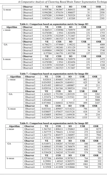
Table 6 : Comparison based on segmentation metric for image H3
Algorithm Observer VE COS SO USR OSR
c-mean Observer1 0.384515 1.938986 1.769979 195 1475 Observer2 0.478308 1.9541 1.824456 131 1753 Observer3 0.312978 1.922549 1.712467 271 1248 Observer4 0.218055 1.861523 1.513467 569 936
Observer VE COS SO USR OSR
GA Observer1 0.786271 1.974969 1.90232 80 4089 Observer2 0.875037 1.982481 1.931129 50 4401 Observer3 0.698804 1.990283 1.961506 34 3740 Observer4 0.57504 1.961791 1.852789 157 3253
Observer VE COS SO USR OSR
k-mean Observer1 0.384515 1.938986 1.769979 195 1475 Observer2 0.478308 1.9541 1.824456 131 1753 Observer3 0.312978 1.922549 1.712467 271 1248 Observer4 0.218055 1.861523 1.513467 569 936
Table 7 : Comparison based on segmentation metric for image H4
Algorithm Observer VE COS SO USR OSR
c-mean Observer1 0.02814 1.404603 0.507213 802 27 Observer2 0.034503 1.464439 0.604911 625 30 Observer3 0.431493 1.889163 1.600887 45 211 Observer4 0.020316 1.261266 0.300524 1541 27
Observer VE COS SO USR OSR
GA Observer1 1.163623 1.751299 1.203329 335 3282 Observer2 1.233474 1.793488 1.315341 241 3368 Observer3 1.654468 2 2 0 3888 Observer4 0.973981 1.569032 0.79531 899 3107
Observer VE COS SO USR OSR
k-mean Observer1 0.033161 1.409057 0.514232 796 32 Observer2 0.038857 1.470437 0.615126 618 34 Observer3 0.436805 1.903941 1.649438 39 216 Observer4 0.023979 1.264142 0.304336 1535 32
Table 8 : Comparison based on segmentation metric for image H5
Algorithm Observer VE COS SO USR OSR
c-mean Observer1 1.561763 1.808411 1.356863 246 8275 Observer2 1.547775 1.796421 1.32342 273 8245 Observer3 1.441772 1.804577 1.346097 333 7942 Observer4 1.572131 1.788933 1.302872 267 8315
Observer VE COS SO USR OSR
GA Observer1 0.516971 1.548287 0.755365 580 693 Observer2 0.480643 1.551081 0.760679 602 658 Observer3 0.337311 1.512911 0.689818 830 523 Observer4 0.530428 1.546245 0.751495 574 706
Observer VE COS SO USR OSR
Figure 3 : volume error for Image H1and H2
Figure 4 : volume error for Image H3 andH4
IV. CONCLUSION
In this work k-mean, c-mean and GA based clustering are studied, implemented and analyzed individually based on the same data set. By analyzing the facts, it can be concluded that clustering efficiency is totally depends on characteristics of data. Different clustering approach gives best result for different images. Therefore only clustering based approach alone can not give best result, rather some additional approach along with clustering should be adopted for getting the best result in every case.
R
EFERENCES[1]. Zaitoun, N. M., & Aqel, M. J. (2015). Survey on Image Segmentation Techniques. Procedia Computer Science, 65, 797–806. https://doi.org/10.1016/j.procs.2015.09.027
[2]. R. Xu and D. Wunsch, Clustering, IEEE Press Series on Computational Intelligence, Wiley, 2008. [3]. Wu, M.-N., Lin, C.-C., & Chang, C.-C. (2007). Brain Tumor Detection Using Color-Based K-Means
Clustering Segmentation. In Third International Conference on Intelligent Information Hiding and Multimedia Signal Processing (IIH-MSP 2007). IEEE. https://doi.org/10.1109/iihmsp.2007.4457697 [4]. Juang, L.-H., & Wu, M.-N. (2010). MRI brain lesion image detection based on color-converted K-means
clustering segmentation. Measurement, 43(7), 941–949. https://doi.org/10.1016/j.measurement.2010.03.013
[5]. Vijay, J., & Subhashini, J. (2013). An efficient brain tumor detection methodology using K-means clustering algoriftnn. In 2013 International Conference on Communication and Signal Processing. IEEE. https://doi.org/10.1109/iccsp.2013.6577136
[6]. Singh, G., & Ansari, M. A. (2016). Efficient detection of brain tumor from MRIs using K-means segmentation and normalized histogram. In 2016 1st India International Conference on Information Processing (IICIP). IEEE. https://doi.org/10.1109/iicip.2016.7975365
[7]. Gopal, N. N., & Karnan, M. (2010). Diagnose brain tumor through MRI using image processing clustering algorithms such as Fuzzy C Means along with intelligent optimization techniques. In 2010 IEEE International Conference on Computational Intelligence and Computing Research. IEEE. https://doi.org/10.1109/iccic.2010.5705890
[8]. Hsieh, T. M., Liu, Y.-M., Liao, C.-C., Xiao, F., Chiang, I.-J., & Wong, J.-M. (2011). Automatic segmentation of meningioma from non-contrasted brain MRI integrating fuzzy clustering and region growing. BMC Medical Informatics and Decision Making, 11(1). https://doi.org/10.1186/1472-6947-11-54
[9]. Parveen, & Singh, A. (2015). Detection of brain tumor in MRI images, using combination of fuzzy c-means and SVM. In 2015 2nd International Conference on Signal Processing and Integrated Networks (SPIN). IEEE. https://doi.org/10.1109/spin.2015.7095308
[10]. Shasidhar, M., Raja, V. S., & Kumar, B. V. (2011). MRI Brain Image Segmentation Using Modified Fuzzy C-Means Clustering Algorithm. In 2011 International Conference on Communication Systems and Network Technologies. IEEE. https://doi.org/10.1109/csnt.2011.102
[11]. A.Rajendran, & Dhanasekaran, R. (2012). Fuzzy Clustering and Deformable Model for Tumor Segmentation on MRI Brain Image: A Combined Approach. Procedia Engineering, 30, 327–333. https://doi.org/10.1016/j.proeng.2012.01.868
[12]. Nithila, E. E., & Kumar, S. S. (2016). Segmentation of lung nodule in CT data using active contour model and Fuzzy C-mean clustering. Alexandria Engineering Journal, 55(3), 2583–2588. https://doi.org/10.1016/j.aej.2016.06.002
[13]. Maulik, U., & Bandyopadhyay, S. (2000). Genetic algorithm-based clustering technique. Pattern Recognition, 33(9), 1455–1465. https://doi.org/10.1016/s0031-3203(99)00137-5
[14]. Chandra, G. R., & Rao, K. R. H. (2016). Tumor Detection In Brain Using Genetic Algorithm. Procedia Computer Science, 79, 449–457. https://doi.org/10.1016/j.procs.2016.03.058