An Improved Shuffled Frog Leaping Algorithm with Single Step Search Strategy and Interactive Learning Rule for Continuous Optimization

An Improved Shuffled Frog Leaping Algorithm

with Single Step Search Strategy and Interactive

Learning Rule for Continuous Optimization

Deyu Tang

College of Medical Information and Engineering, GuangDong Pharmaceutical University, GuangZhou, China Email:[email protected]

Yongming Cai

Dept of Computer, College of Medical Information and Engineering, GuangDong Pharmaceutical University, GuangZhou, China

Email: [email protected]

Jie Zhao

Department of information management engineering, School of Management, Guangdong university of technology, GuangZhou, China

Email: [email protected]

Abstract—Shuffled frog-leaping algorithm (SFLA) is a heuristic optimization technique based on swarm intelligence that is inspired by foraging behavior of the swarm of frogs. The traditional SFLA is easy to be premature convergence. So, we present an improved shuffled frog-leaping algorithm with single step search strategy and interactive learning rule(called ‘SI-SFLA’). Single step search strategy enhances exploring ability of algorithm for higher dimension and interactive learning rule strengthens the diversity of local memeplexe. The effectiveness of the method is tested on many benchmark problems with different characteristics and the results are compared with other algorithms including PSO,SFLA,DE and TLBO. The experimental results show that SI-SFLA has not only a promising performance of searching for accurate solutions, but also a fast convergence rate, which are evaluated using benchmark functions.

Index Terms—shuffled frog-leaping algorithm, single stepsearch strategy, interactive learning rule, continuous optimization, swarm intelligence

I. INTRODUCTION

Evolutionary computing (EC) is an exciting development in computer science. Over the past several decades, people have developed many optimization computation methods to solve complicated global optimization problems such as genetic algorithm (GA) inspired by the Darwinian law of survival of the fittest [1], particle swarm optimization (PSO) inspired by the social behavior of bird flocking or fish schooling [2][3]; ant colony optimization (ACO) inspired by the foraging behavior of ant colonies [4]; and biogeography-based optimization (BBO) inspired by the migration behavior of island species [5][6]; Differential Evolution (DE) [7][8]

which is similar to GA with specialialized crossover and selection method; Teaching-Learning-based Optimization algorithm [9][10][11][12] which imitates the process of the teaching about teacher and students; Shuffled frog leaping algorithm (SFLA) which imitates the foraging behavior of frogs; all these algorithms can be called evolutionary algorithm or swarm intelligence optimization algorithm. Developed by Eusuff and Lansey in 2003, the shuffled frog-leaping algorithm [16] (SFLA) is a meta-heuristic optimisation method spired from the memetic evolution of frogs seeking food in a pond, which combines the advantages of the genetic-based MA [17] and the social behaviour-based particle swarm optimisation(PSO). Memetic algorithms (MAs) are a special class of heuristic searching methods that are derived from the models of adaptation in natural systems that combine the evolutionary adaptation of a population with individual learning within the lifetimes of their members. MAs are based on evolution of memes carried by the interactive individuals. The term memetic algorithm comes from ‘meme’, which is a transmittable information pattern that is replicated by infecting the objects ’s minds and altering their behavior in a parasitic manner. The remarkable characteristic of MAs is that all memes are allowed to gain some experience through a local search before being involved in the evolutionary process.

In general, the SFLA includes two alternating processes: local exploration in the submemeplex and global information exchange among all memeplexes. Local exploration uses the search strategy of PSO and shuffled method was used for global information exchange.

In SFLA algorithm, the whole position vector of frog was updated simultaneously, rather than each

component of the position vector was updated independently in each iteration, so it is difficult to find the best solution in higher dimensional space. So, according to the correlation of data set, the vector can be divided into several sub-vectors, each sub-vector can be updated in cycle. At the same time, the frog analyzes the state of position before the new position was updated, then determines the updating speed of the sub-vector during the updating process.

As everyone knows, in real life, during the learning process of student in a class, in general, there are two ways. one is that the teacher guides the student to access to the new knowledge, the second method is through the interaction between the students, which can improve the learning effect. Therefore, we introduce this interactive learning method into our algorithm. One frog in the population can be associated with arbitrary two frogs in population learning from each other, which improves the global searching ability of SFLA.

In this paper, we introduce an improved SFLA algorithm with a strong searching capabilities. A singal step strategy was used to improve the local exploration and an interactive learning rule was utilized to enforce the global searching capability. The rest part of the paper is organized as follows. In Section 2, a brief introduction of SFLA is given. The improved SFLA is introduced in Section 3. In Section4, Experiments show the result of our algorithm.

II. SFLA ALGORITHM

Shuffled frog leaping algorithm simulates the process of a group of frogs looking for food. The population was classified into some memeplexes (community), in each memeplex, frogs exchange their thoughts. SFLA is a heuristic method combined with the shuffled strategy and the local search strategy. The local search strategy makes the thought of frog spread in local search space and the shuffled strategy exchanges the idea of local memeplex. In the shuffled frog leaping algorithm, a group of frogs have the same structure which is composed of solution(position) and food(fitness). According to a certain strategy, frogs of memeplex implement local search in the solution space. After the number of local search step, thought in the shuffled process was exchanged. Local search and shuffled process continue until the definition of convergence condition was satisfied [15] [16] [17].

A balance strategy of global information exchange and the local search makes the algorithm can jump out of local optimum solution and search toward the global optimum direction, which is the most important characteristics of shuffled frog leaping algorithm. In SFLA, each memeplex carry out the local search respectively, the worst individual

Q

w, through the

memetic evolution close to the local best individual

Q

bor

the global individual

Q

g . When the local search is

executed to a certain stage, frogs in each memeplex communicate to implement shuffled process. The basic SFLA algorithm is as follows:

a). parameter settings: population size, numbers of memeplexes, maximum of local search iterations, number of global iterations.

b). generates an initial population.

c). determine the fitness function: F(x), used to evaluate the quality of the individuals.

d). in the global iteration process, the frog was arranged in descending order by whose fitness, and determine the global optimal solution

Q

g, if it meet the convergence

condition, then stop the execution; otherwise, proceed to the next step.

e). frog population was divided: the frog population was divided into m memeplexes, each memeplex contains n frogs, and the number of the population meet T=m

×

n; then, the first frog is divided into the first memeplex, the second frog was divided into the second memeplex, ... , The M frog was divided into the M memeplex, the m+1frog was divided into the first memeplex, the m+2frog was divided into the second memeplex, and so on, until the whole frogs was division. That is:

( 1)

{ |1 }

t t m r

Q = Q_{+ −} ∈T ≤ ≤r n ,

(1

≤ ≤

t

m

)

(1)

f). each memeplex implement local search in the number of the iterations.

(1) determine

Q

w,

Q

b , according to the following

formula to update, where

rand

∈

(0,1]

,

r

is a

constant.

(

b w

)

D

= •

r rand

•

Q

−

Q

(2)

( ) , [ min, max]

w new w

Q =Q +D D∈ D D (3)

(2) If a better solution was produced, then

Q

w was

updated by

Q

w new( ) ;else

Q

b was replaced by

Q

g

according to the formula (1)(2).if

Q

wwas not improved,

then a new solution

Q

'w new( ) _{was produced randomly, if}

it is better, then the

Q

w was updated by

Q

w new( )_.

III. IMPROVED SFLA ALGORITHM

A. Single step Search Strategy

For example, on three dimensional function Sphere

2 2 2

1 1 2 3

f

=

x

+ +

x

x

, the global optimum value is (0, 0, 0),

the initial value of solutions was set (10, 10, 10), the fitness value is 300. Give a random perturbation variable value (1, 0, 1), the initial value was updated to the value (11, 0, 11), and the fitness value is 242.The fitness (242) of the updated solution is less than the initial fitness value(300). So, we can see that, in the next iteration, the solution would be some extent to move toward (11, 0, 11). At this time, although the second dimension moves to the global optimum direction, but the first and third dimension move away from the global optimum. Therefore, for high-dimensional functions, general SFLA algorithm is very difficult to find the best direction of all dimension. In order to solve this problem, the search space of the frogs was divided into several low dimensional space, in specific application, according to the dependence analysis of data set, we can decide the segmentation of the data dimension. The worst frog uses a single step search strategy for each low dimensional space. If a new frog abtains a better solution than the worst frog, then the worst frog position was updated by it, else the worst frog position was updated by it with a small search step. That is as follows formula (4)(5):

( ) . .( ( ) ( ))

temp w w

Q =Q t +c rand Qbest t −Q t (4)

{

( 1) , . .

( 1) . ,

w temp temp w

w temp

Q t Q Q fitess Q fitness Q t rand Q otherwise

+ = ≤

+ = (5)

B. Interactive Learning Rule

In real life, interactive learning is common. For example, students in a class often learn new knowledge through mutual discussions and exchange information for each other [9]. SFLA is a swarm intelligence algorithm. In each memeplex(community), the worst frog learns toward the best frog. In traditional SFLA, between memeplexes, the frogs were only shuffled, but they do not learn from each other. This reduces the efficiency of learning. Therefore, we use an Interactive learning rule. Firstly, we let frogs in each memeplex complete a local search; Secondly, frogs in all memeplexes learn from each other to exchange information, then was shuffled. Interactive learning method strengthens the internal information exchange, enhances the global searching ability of the algorithm. Two frogs Qa, Qbj was choosed randomly in population. The Interactive learning rule is

as follows:

{

( 1) ( ) .( ( )), . .

( 1) ( ) .( ( ) ),

a a b a j i

a a a b

Q t Q t rand Q Q t Q fitness Q fitness

Q t Q t rand Q t Q otherwise

+ = + − ≤

+ = + − (6)

The improved algorithm as shown in Figure 1. Figure 1 shows frog’s searching process with a number of population 30. The population was divided into 5 memeplexes, each memeplex has 6 frogs. The frogs in each column of table belongs to the same memeplex. Frogs implement local search in each memeplex, for example: the first column of table with arrows shows that frogs in the same memeplex use a one-step search strategy for local search. Interactive learning rule represents the frogs among all the memeplexes (population) communicate between each other. For example, to update the position of the frog

Q

i m j+ _{( 1)}− ,

randomly choose another different frog

Q

u m v+ _{( 1)}− in the

whole population respectively, these two frogs communicate with each other and determine how to update it according to the formula (6). The process is as Fig.1.

Fig.1 the searching process of SI-SFLA

The pseudo-code is as follows:

1

Q

Q

₂

Q

₃

Q

₄

Q

₅

1 5

Q

₊

1 2 5

Q

_{+ ×}

Q

_{i m j+ ( 1)−}

( 1)

u m v

Q

_{+ −}

IV. EXPERIMENTS AND RESULTS

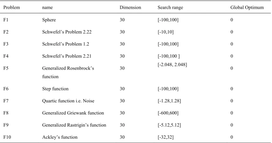
A. Test Functions

In this paper, ten widely used benchmark continuous functions [18] shown in Table 1 with high complexity are tested. Also different benchmark problems are considered having different characteristics such as multimodality. A function is multimodal if it has two or more local optima in their solution space. Complexity increases when the local optima are randomly distributed. Moreover, complexity increases with the increase in the dimensionality.F8~F10 function are multimodality. F7 function is quartic function i.e. Noise. Initialisation dimension, search range and global optimum of these ten functions are given in Table1.The SI-SFLA algorithm is compared with standard PSO [2], standard SFLA [16],

standard DE [7] and TLBO [9] to search for the global minima in the solution space. Details of benchmark functions are given in the appendix.

B. Initialisation Parameters Setting

The global parameter is set as follows:the population size is 50 and dimension is 30. For the basic PSO, the acceleration coefficient is set as c1 = c2 = 2, the inertia weight w decreases linearly from 0.9 to 0.4. For DE, the coefficient is set as F=0.5, CR=0.5; For the basic shuffled frog-leaping algorithm, there are 10 memeplexes, each containing 5 frogs. The local exploration in each submemeplex is executed for 5 iterations. The parameters settings for SI-SFLA are the same as those of SFLA, with the searching scale parameter c equal to 2.0; there is not

other parameter to be set for TLBO algorithm. Especially the global iteration number is 1000 for PSO,DE and TLBO, and 200 for SFLA and SI-SFLA, because the local iteration number of SFLA and SI-SFLA are 5, then total iteration number of SFLA and SI-SFLA are 5*200=1000.

C. Test Results and Discussion

To test the performance of the improved SFLA (SI-SFLA), ten benchmark functions listed in Table 1 are used here for comparison with PSO, DE, SFLA and TLBO. We had 50 trial runs for every instance and recorded minimum of best fitness, maximum of best fitness, midian of best fitness, mean best fitness and standard deviation.

As shown in Table 2, SI-SFLA is able to evolve in a very efficient manner. Convergence rates of SI-SFLA were strikingly higher than those of PSO, DE, SFLA and TLBO. SI-SFLA also demonstrated its robustness by very consistent performances: across all of the randomly initialized runs on the same test function, SI-SFLA always showed very similar evolution speed and converged to the same point or a small region, whereas for PSO, DE SFLA and TLBO, they sometimes had very diverse behaviors resulting from the random initialization.

Because each function in f1~f7 has only a single optimal solution on origin, which usually is employed to test the local search ability of the algorithm. Thus from the result, we can see that SI-SFLA has stronger local search ability than PSO, DE, SFLA and TLBO. Especially, f3 function (Schwefel’s Problem 1.2) has a flat area, so many algorithms do not easy to get its optimal solution. The result in Table2 show that SI-SFLA has a highest accuracy than PSO,DE,SFLA and TLBO.TLBO works better than PSO, DE, SFLA, but it is not stable than SI-SFLA. F8, F9 and F10 function are both multi-modal and usually tested for comparing the global search ability of the algorithm. On F8, F9 and F10 function, the SI-SFLA has better performance than PSO,DE,SFLA and TLBO algorithm; particularly, SI-SFLA can also find the optimal or closer-to-optimal solutions on the complex multimodal functions.

1.Initialize parameters: m, n, p=m*n, etc.

Generate population(represented by P frogs ) randomly;

2.Evaluate fitness of each frog;

3.While( convergence criteria is satisfied) 4.{

5. Sort P frogs in descending order;

(Shuffled all frogs(construct n groups and each groups has m frogs );

6.For groups 7.{

8.Get the worst frog Qw and the best frog Qb in this group;

9.Qtemp =Qw(t)+c.rand.(Qbest(t)-Qw(t) ) ; 10. For each Dimension

11. If Qtemp.fitness < Qw(t).fitness 12. Qw(t+1)= Qtemp ;

13. Else

14. Qw(t+1)= rand.*Qtemp ; 15. End ;

16.end

17.get new frog using mutation; 18.if Qnew.fitness<Qw(t).fitnes 19. Qw=Qnew;

20. end 21.}

22.For each frog in population 23.{

24. get two frogs Qa, Qb randomly from population; 25. Q1=Qa(t)+rand.(Qb-Qa) ;

26. Q2= Qa(t)+rand.(Qa-Qb) ; 27. If Q1.fitness<Q(t).fitness 28. Q(t+1)=Q1;

29. Else

30. Q(t+1)=Q2; 31. End

TABLE 1

DETAILSOFBENCHMARKFUNCTIONS

Problem name Dimension Search range Global Optimum

F1 Sphere 30 [-100,100] 0

F2 Schwefel’s Problem 2.22 30 [-10,10] 0

F3 Schwefel’s Problem 1.2 30 [-100,100] 0

F4 Schwefel’s Problem 2.21 30 [-100,100 ] 0

F5 Generalized Rosenbrock’s function

30 [-2.048, 2.048] 0

F6 Step function 30 [-100,100] 0

F7 Quartic function i.e. Noise 30 [-1.28,1.28] 0

F8 Generalized Griewank function 30 [-600,600] 0

F9 Generalized Rastrigin’s function 30 [-5.12,5.12] 0

F10 Ackley’s function 30 [-32,32] 0

TABLE 2

COMPARISISION OF RESULTS FOR THE MIN,MAX,MIDIAN,MEAN AND THE STANDARD DEVIATION FRO PSO,SFLA,DE,TLBO AND SI-SFLA.

PSO SFLA DE TLBO SI-SFLA

F1 min Max Midian Mean SD. 0.7101 33.9085 5.6048 7.2682 6.2093 7.0825e-005 1.4129 4.0592e-004 0.0610 0.2302 2.2351e-011 2.2091e-010 4.4524e-011 5.8090e-011 3.8643e-011 2.5400e-015 14.2100 2.6605e-005 0.4735 2.2540 9.1988e-093 5.0804e-090 4.0838e-091 9.4713e-091 1.2209e-090 F2 min

Max Midian Mean SD 0.0100 0.3256 0.0494 0.0728 0.0751 1.2102e-006 100.0000 7.2865e-006 4.0002 19.7948 4.7970e-013 1.1728e-011 2.0384e-012 2.4012e-012 1.9589e-012 2.1934e-012 1.0815e+006 5.5212e-007 2.1629e+004 1.5294e+005 1.2287e-094 5.0111e-092 3.2693e-093 5.9400e-093 8.2468e-093 F3 min

Max Midian Mean SD 4.3075e+004 1.6568e+005 7.7664e+004 8.4972e+004 2.9328e+004 3.7439e+004 1.6784e+005 7.7712e+004 8.0585e+004 2.8036e+004 1.3528e+005 4.7575e+005 2.9498e+005 2.9151e+005 7.9253e+004 3.2865e-010 2.8937e+005 0.5759 1.0295e+004 4.3603e+004 4.2474e-016 645.9814 0.5302 48.9997 115.4962 F4 min

Max Midian Mean SD 11.2857 27.6603 21.2735 20.5526 3.7755 3.0528 25.0490 14.4736 14.2677 5.0859 0.9726 2.1760 1.4421 1.4777 0.3142 1.0945e-007 0.7453 0.0158 0.0720 0.1436 3.1176e-072 7.6636e-070 3.0160e-071 6.5088e-071 1.2422e-070 F5 min

Max Midian Mean SD 16.9985 145.7181 29.2503 41.8042 27.6833 18.6618 83.4157 28.5246 35.0193 18.8570 23.3310 25.6784 24.4105 24.4319 0.5520 28.7832 7.5675e+003 28.9009 179.6730 1.0661e+003 26.2041 28.5672 27.1582 27.1621 0.6455 F6 min

Max Midian Mean SD 2 34 11 11.9400 6.6774 0 170 1 5.5200 24.8261 0 0 0 0 0 0 20 0 1.2800 3.3444 0 0 0 0 0 F7 min

Max Midian Mean SD 0.0478 0.2660 0.1316 0.1325 0.0453 0.0158 0.2550 0.0434 0.0567 0.0427 0.0100 0.0366 0.0237 0.0237 0.0059 2.3995e-005 0.0045 6.6088e-004 9.0397e-004 8.9015e-004 1.1186e-005 8.6906e-004 2.2484e-004 2.5737e-004 1.7105e-004 F8 min

Max Midian 0.8571 1.1425 1.0370 1.4462e-004 1.0344 0.0028 5.4495e-011 1.0280e-007 3.1306e-010 2.0017e-013 1.3998 1.1138e-004 0 0 0

Mean

SD 1.0292 0.0529 0.0533 0.1674 3.5514e-009 1.5102e-008 0.0915 0.2771 0 0 F9 min

Max Midian Mean SD

33.4843 116.9836 64.3820 65.8825 17.8519

27.6249 226.2016 81.5295 95.3020 53.0519

98.1627 145.0373 134.4844 132.0604 9.7593

1.2260e-010 165.9932 7.5345e-004 9.2961 34.6402

0 0 0 0 0 F10 min

Max Midian Mean SD

0.7373 3.1276 1.9979 1.9632 0.6116

0.0029 4.6982 0.9379 1.2461 1.2581

1.1695e-006 4.1530e-006 2.0644e-006 2.2340e-006 7.0297e-007

3.6651e-008 5.4371 0.0028 0.2293 0.8739

8.8818e-016 8.8818e-016 8.8818e-016 8.8818e-016 0

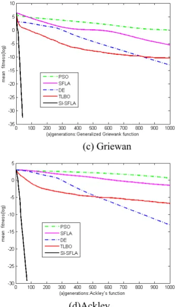
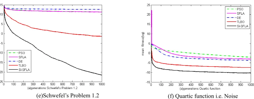
Fig 2 gives the comparison of convergence processes of SI-SFLA, PSO, SFLA, DE and TLBO in the above six benchmark functions (F1, F3, F7, F8, F9, F10) averaged on 50 trial runs, when the population size is 50 and the maximum generation is 1000 according to the dimension 30. For SFLA and SI-SFLA, the maximum generation=5*200. (local iteration number is 5 and global iteration number is 200). The result show that SI-SFLA has a quick convergence speed than PSO,SFLA,DE and TLBO, especially, for F1, F8, F9, F10 function, SI-SFLA

obtains global solution or closer-to-global solution in iteration 100.

D. Change of Difference in Efficiency with Increasing Dimensionality

To further demonstrate its efficiency and effectiveness on high-dimensional problems, we also compared SI-SFLA with PSO, SFLA, DE and TLBO. SI-SFLA has a more smaller value of the mean and the standard deviation than PSO, SFLA, DE and TLBO, when the dimension is 10, 30 and 50 as TABLE 3~6.

(a)Sphere (c) Griewan

(e)Schwefel’s Problem 1.2 (f) Quartic function i.e. Noise

Fig 2 Convergence curve for different benchmark problems

TABLE 3

NUMERICAL EXPERIMENT RESULTS OF SPHERE FUNCTION(F1)

Dimension PSO SFLA DE TLBO SI-SFLA

10Mean

SD 5.7236e-012 1.3761e-011 2.7017e-025 7.7906e-025 1.2459e-045 2.5355e-045 0.0428 0.1863 5.6119e-110 1.2353e-109 30Mean

SD 7.2682 6.2093 4.6363e-005 2.8341e-004 5.8090e-011 3.8643e-011 0.4735 2.2540 9.4713e-091 1.2209e-090 50Mean

SD 524.7095 196.9751 32.6081 92.6275 0.0038 0.0013 0.6408 3.4093 4.8316e-086 6.0995e-086

TABLE 4

NUMERICAL EXPERIMENT RESULS OF GENERALIZED RASTRIGIN’S FUNCTION(F9)

Dimension PSO SFLA DE TLBO SI-SFLA

10Mean

SD 3.2778 1.6819 7.2302 3.6425 3.8369e-015 1.4140e-014 2.2046 5.9969 0 0 30Mean

SD 65.8825 17.8519 59.7707 24.0783 132.0604 9.7593 9.2961 34.6402 0 0 50Mean

SD 195.5192 38.6663 298.5764 99.2877 335.7978 13.9482 4.0913 19.6936 0 0

TABLE 5

NUMERICAL EXPERIMENT RESULTS OF ACKLEY’S FUNCTION9F(10)

Dimension PSO SFLA DE TLBO SI-SFLA

10Mean

SD 6.8402e-007 6.5761e-007 0.3334 0.5923 4.4409e-015 0 0.3614 1.1992 8.8818e-016 0 30Mean

SD 1.9632 0.6116 1.1479 1.2890 2.3458e-006 7.5809e-007 0.2293 0.8739 8.8818e-016 0 50Mean

SD 6.1583 0.8369 3.8771 2.7107 0.0154 0.0031 19.6936 1.3180 8.8818e-016 0

TABLE 6

NUMERICAL EXPERIMENT RESULTS OF GENERALIZED GRIEWANK FUNCTION(F8)

Dimension PSO SFLA DE TLBO SI-SFLA

10Mean

SD 0.1129 0.0711 0.0464 0.0275 2.7145e-004 0.0019 0.2009 0.2608 0 0 30Mean

SD 1.0292 0.0529 0.0533 0.1674 3.5514e-009 1.5102e-008 0.0915 0.2771 0 0 50Mean

SD 6.0022 2.4769 1.2027 0.7862 0.0063 0.0037 0.1114 0.3256 0 0

Especially, SI-SFLA has a good fitness for F8, F9, F10 function, which have many local best fitness, regardless of dimension is 10, 30 or 50. That is to say, our algorithm

has a good robustness.

V. CONCLUSION

SFLA algorithm was an heuristic algorithm which combined PSO[19][20][21] with MA algorithm.This paper presents a novel improved SFLA algorithm (called SI-SFLA) to improve the stability and global search ability for high-dimensional continuous function optimisation. Single step search strategy and interactive learning rule was introduced to improved SFLA Algorithm. Single step search strategy is based on multidimensional data correlation to determine the search direction, which improved the search accuracy of SFLA algorithm, and interactive learning rule makes all the frogs find new important information which strengthen the global searching ability of the SFLA algorithm. The performance of the proposed SI-SFLA method is checked with the recent and well-known optimization algorithms such as PSO, SFLA, DE, TLBO, etc. by experimenting with different benchmark problems with different characteristics like, multimodality and dimensionality. The effectiveness of SI-SFLA method is also checked for different performance criteria, like midian, standard deviation, mean solution, average function evaluations required, convergence rate, etc. The results show better performance of SI-SFLA method over other natured-inspired optimization methods for the considered benchmark functions. This method can be used for the optimization of engineering design applications.

APPENDIX BENCHMARK FUNCTION 1. F1 Sphere

₁ 2 1 n i i

f

x

=

=

∑

2. F2 Schwefel’s Problem 2.22

₂ 2 30

1 1

( )

n

|

i

|

| |

i

i i

f x

x

x

= =

=

∑

+

∏

3. F3 Schwefel’s Problem 1.2

2

3

1 1

( )

n

(

i j

)

i j

f x

x

= =

=

∑ ∑

4. F4 Schwefel’s Problem 2.21

f

4( ) max{| |}, [1, ]

x

=

x

i

i

∈

n

5. F5 Generalized Rosenbrock’s function

1

2 2 2

1 1

5( )

n

100 (

i i

) (1

i

)

i

f

x

x

x

x

−

+ =

=

∑

•

−

+ −

6. F6 Step function

6. 2

1

6( )

n

(

i

0.5 )

i

f

x

x

=

=

∑

+

7. F7 Quartic function i.e. Noise

4

1

7( )

n i

[0,1)

i

f

x

ix

random

=

=

∑

+

8. F8 Generalized Griewank function

2

1 1

1

8( )

cos( ) 1

4000

n n i i i i

x

f

x

x

i

= =

=

∑

−

∏

+

9. F9 Generalized Rastrigin’s function 2

1

9( ) n ( i 10cos(2 i) 10) i

f x x

π

x

=

=

∑

− +

10. F10 Ackley’s function 2

1 1

1 1

10( ) 20exp 0.2 n i exp n cos(2 i) 20

i i

f x x x e

n = n = π

⎛ ⎞ _{⎛ ⎞}

= − ⎜_⎜− ⎟_⎟− _{⎜ ⎟}+ +

⎝ ⎠

⎝

∑

⎠

∑

ACKNOWLEDGMENT

This paper has been supported by Guangdong Province Natural Science Doctoral start-up fund project (S2011040004285); Humanities and Social Science Youth Fund project of Education Ministry (10YJCZH234); the subject of Ideological and political education in Guangdong Province (NO.2011ZZ012); Research on Guangdong Province college Party Construction, (NO.2012BKZZB12). Guangdong Province Science and technology plan project (2012B031000018)

REFERENCES

[1] D.E. Goldberg, “Genetic Algorithms in search Optimization and Machine Learning, ” Addison-Wesley,

Reading, MA, 1989.

[2] J. Kennedy, R. Eberhart, “Particle swarm optimization,”in:

Proceedings of IEEE International Conference On Neural Network, 1995, pp. 1942-1948.

[3] Xingjuan Cai, Zhihua Cui, Jianchao Zeng, Ying Tan, “Dispersed particle swarm optimization,”Information Processing Letters, 105 (2008) 231-235

[4] M. Dorigo, Optimization, “Learning and Natural Algorithms,”Ph.D. Thesis, Politecnico di Milano, Italy,

1992.

[5] D. Simon, “Biogeography-based optimization, ”IEEE Transactions on Evolutionary Computation (12) (2008)

702-713.

[6] D. Simon, M. Ergezer, D. Du,“Population distributions in biogeography-based optimization algorithms with elitism, ”in: IEEE Conference on Systems, Man, and

Cybernetics, 2009, pp. 1017-1022.

[7] R. Storn and K. Price, “Differential evolution - A simple and efficient adaptive scheme for global optimization over continuous spaces,” ICSI Tech. Rep. TR-95-012 (1995).

[8] R. Storn and K. Price, “Differential evolution - A simple and efficient heuristic for global optimization over continuous spaces,” J. Global Optimization 11 (1997)

341-359.

[9] R.V. Rao, V.J. Savsani, D.P. Vakharia, “Teaching-Learning-Based Optimization,”Information Sciences, 183 (2012) 1-15

[10]TaherNiknam, Rasoul Azizipanah-Abarghooee, Mohammad Rasoul Narimani, “A new multi objective optimization approach based on TLBO for location of automatic voltage regulators in distribution systems,”Engineering Applications of Artificial Intelligence 2012, 25, 1577-1588.

[12]TaherNiknam, Rasoul Azizipanah-Abarghooee, Mohammad Rasoul Narimani, “A new multi objective optimization approach based on TLBO for location of automatic voltage regulators in distribution systems,”Engineering Applications of Artificial Intelligence 2012, 25, 1577-1588.

[13]M. Eusuff, K. Lansey, “Optimization of water distribution network design using the shuffled frog leaping algorithm, ”

Journal of Water Resource Plan and Management 129 (3)

(2003) 10-25.

[14]Q. Y. DUAN, V. K. GUPTA, S. SOROOSHIAN, “Shuffled Complex Evolution Approach for Effective and Efficient Global Minimization, ”JOURNAL OF OPTIMIZATION THEORY AND APPLICATIONS: Vol. 76,

No. 3, (1993)MARCH.

[15]Thai-Hoang Huynh, “A modified shuffled frog leaping algorithm for optimal tuning of multivariable PID controllers,” in: Proceedings of International Conference on Information Technology(ICIT 2008), Singapore, 2008,

pp.21-24.

[16]J.P. Luo, M.R. Chen, X. Li, “A novel hybrid algorithm for global optimization based on EO and SFLA, ”in:

Proceedings of the Fourth IEEE conference on Industry electronics and applications (ICIEA2009), Xi’an, China,

2009, pp. 1935-1939.

[17]Xia Li, Jianping Luo, Min-Rong Chen, Na Wang. “An improved shuffled frog-leaping algorithm with extremal optimisation for continuous optimisation,” Information Sciences 192 (2012) 143-151

[18]Han Huang, Hu Qin, Zhifeng Hao, Andrew Lim. “Example-based learning particle swarm optimization for continuous optimization,” Information Sciences. 182 (2012)

125-138.

[19]Liangyou SHU, Lingxiao YANG, “A Modified PSO to Optimize Manufacturers Production and Delivery”,

JOURNAL OF SOFTWARE, VOL. 7,pp,2325-2332,2012.

[20]Shengli Song, Yong Gan, Li Kong ,Jingjing Cheng, “A Novel PSO Algorithm Based on Local Chaos & Simplex Search Strategy and its Application, ” JOURNAL OF SOFTWARE, VOL. 6, pp.604-611, 2011.

[21]Weitian Lin, Xingsheng Gu, Zhigang Lian, Yufa Xu,Bin Jiao, “A Self-Government Particle Swarm OptimizationAlgorithm and Its Application in TexacoGasification, ” JOURNAL OF SOFTWARE, VOL. 8,

472-479 ,2013.

Deyu Tang was born in Jilin Province,

China in 1978. He received his degree of Master in Computer software and theory in 2004 at South China University of Technology, China. Currently he is working on his doctoral degree in computer application at South China University of Technology, China. He is a Docent in College of Medical Information and Engineering at GuangDong Pharmaceutical University, Guangzhou, China. He has published at least 5 articles. Two of them has been published in Computer engineering and Applications. Three of them can be indexed by EI. His interest is in studying data mining, Bioinformatics, Swarm intelligence.

Yongming Cai was born in GuangDong

Province, China in 1975. He received of Ph.D. in biomedical engineer in 2012 at Sun Yat.sen University, China. Currently, he is an associate professor in College of Medical Information and Engineering at GuangDong Pharmaceutical University, Guangzhou, China. His main research interests are data mining and bioinformatics.