Abstract—Effectiveness and superiority of predictive accuracy of different Data mining (DM) models over the others have traditionally come from results of the empirical studies of DM. Study [4] compared logistic regression, classification tree, neural network, random forest and AdaBoost based on evaluation composite indicators (ECI) built from four parameters like accuracy, interpretability, robustness and speed using four input alternatives (original, aggregated, principal component analysis and stacking based variables), three random indicator weighting criteria and two indicator normalization methods (z-score and min-max). In this study, ECI has been calculated using results from [4] from same four input variable types but using “four plus one” (five) parameters. The fifth parameter of interest (POI) named as Residual Efficiency (RE), has been quantified for this study based on characteristics of interest (COI) described in [10]. Besides, analytical hierarchy process (AHP) of [13] has been used as weighting criteria and step wise utility functions of [12] as normalization technique. Finally we have compared our results with that of [4]. As opposed to study [4], this study has calculated ECIs for all the classifiers used and results have narrower ranges thus are more realistic for comparing the considered classifiers objectively based on type of inputs and POIs.
Index Terms—Knowledge discovery and data mining (KDD), analytical hierarchy process (AHP), evaluation composite indicators (ECI), multi-criteria decision making (MCDM).
I. INTRODUCTION
Data mining (DM) and knowledge discovery in databases (KDD) has been applied to a variety of application domains. Classification methods of data mining has been applied to understand the root causes of Asian financial crisis (twin banking and currency crisis of 1998) [1], credit scoring and evaluation, bankruptcy prediction, insurance underwriting, fraud detection, financial performance prediction, bond rating analysis, credit risk assessment, to forecast daily changes in seven financial stocks‟ prices [2] and other applications in finance [3]. Other important applications cited in this study are to customer churn prediction problem [4] and comparison of social objectives for decision-making in housing corporations [5].
Data modeling or building a model from data is what data mining techniques generate. There are many different data
Manuscript received March 18, 2013; revised June 10, 2013. Views expressed in this paper and all errors and emissions are that of the author and in no case reflect those of LTU or its management.
S. Anjum is with Faculty member (Finance and MIT) for Doctor of Management in Information Technology (DMIT) and Doctor of Business Administration (DBA) programs at College of Management, Lawrence Technological University (LTU), Buell Bldg., M331, 21000 West Ten Mile Road, Southfield, MI 48075-1058, USA (e-mail: anjumsw@ hotmail.com).
mining algorithms with different objectives, different outcomes and with different representation techniques [6]. Data mining taxonomy includes predictive models and descriptive models. Descriptive models include association and clustering and predictive models include classification and regression. Predictive models can be regressor or classifiers [7]. Prediction techniques are similar to classification where unseen data is used to predict the class label of each row of data [8]. Simple parametric to nonparametric statistical methods are used to develop classifiers which are most commonly implemented with neural network (NN), decision tree (DT), Naïve Bayes, logistic regression (LR) or k-nearest- neighbor algorithms. Regarding assessment of classifier, most of comparisons have come from empirical literature where different classifiers were used as a solution approach for a particular problem setting as in [2] and various others (omitted to contain the reference list). Comparisons based on empirical studies reveal that there is no objective conclusion about superiority of one classifier over the other based on types of inputs used and parameters other than accuracy only. Performance of any classifier rather depends on the nature of problem, type of dataset to be used and behavior of variables in that particular problem and has been ranked based on accuracy parameter only in most cases.
II. LITERATURE REVIEW AND DATA DESCRIPTION Besides DM literature cited above, application of certain DM method has been backed by other multi-criteria decision making (MCDM) techniques like Analytical Hierarchy Process (AHP) etc. The use of AHP in a multiplicity of environments is well documented and studies like [3], [8] and [9], besides others, have used AHP in the context of DM. However, all these studies have used AHP for input variable selection. In literature, however, not various studies have been found which have attempted to compare the data mining models based on other discriminate parameters than accuracy only. The study [4] is the one which has attempted a comparison of classifiers by building evaluation composite indicators (ECIs) based on four parameters of Interest (POI) or assessment criteria (AC) in customer churn prediction problem.
In order to rank the DM techniques for classification, various authors have mentioned three POI including accuracy (A), interpretability (I) (or complexity) and speed (S) [7] and ref. [8] has added robustness (R) (or stability or consistency) and lift. The study [10] has quoted that in medical literature, validation ratios for classification algorithm (percentage of correct classified (PCC) for overall
Composite Indicators for Data Mining: A New Framework
for Assessment of Prediction Classifiers
accuracy, sensitivity (true positive rate) and specificity (true negative rate) can be calculated from confusion matrix for a binary classification problem. Receiver operating characteristic (ROC) curve is a commonly used summary for assessing the tradeoff between sensitivity and specificity. It is a plot of the sensitivity versus specificity as we vary the parameters of a classification rule. The Area Under (ROC) Curve (AUC) or c-statistic is a commonly used quantitative summary for accuracy.
This study uses five POIs to arrive at final calculations of ECIs. Four POIs are same as in the reference study [4], which are A (=AUC), I, R (=AUCtest - AUCtrian), and S (or execution time). Here AUCtest (AUCtrain) means AUC for test (train) data. „I‟ of individual classifiers has been defined in ref. [4] on a four point scale based on four categories for null, poor, medium and high interpretability with respective scores of 1, 2, 3 and 4. Based on this yardstick, classification tree (DT) have got high, logistic regression (LR) medium, neural network (NN), AdaBoost (AB) and random forest (RF) have received poor and stacking methodology and PCA have received null category scores. POIs are different from measures of interestingness (MOI) cited in study [6] describing taxonomy of MOI as objective (coverage, support, accuracy) and subjective (unexpected, actionable, novel). Third one is semantics-based MOI.
TABLE I: INFORMATION GATHERED ABOUT COI TO ARRIVE AT INDIVIDUAL
PARAMETERS RESULTS (WITHOUT NORMALIZATION) OF RF-IVSOPAIRS FOR
RESIDUAL EFFICIENCY PARAMETER
COIs RF-IVSO Pairs
RF/OV RF/AV RF/PC RF/SV
COI-1 5 5 5 6
COI-2 6 6 6 6
COI-3 5 5 5 4
COI-4 6 6 6 6
COI-5 5 5 5 6
COI-6 6 6 6 6
COI-7 6 6 6 6
COI-8 6 6 6 6
COI-9 6 5 6 6
COI-10 5 5 5 6
Note: (1) Explanation for cell value of COI-10 versus RF/OP2-SV pair means that because RF is an ensemble method (i.e. present) so it got a score of 3 and as stacking VSO in OP2-SV is also an ensemble method (i.e. present) so it also got a score of 3 and thus the value in respective cell is 6 :) (2) Information in this table has been compiled from these references [4], [6], [10], [9], and [11]
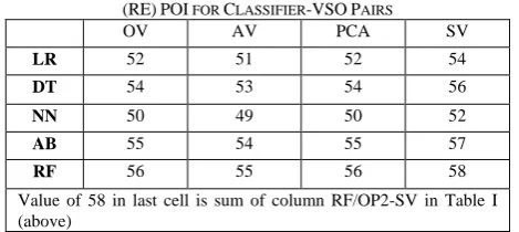
This study has developed a new POI, which has been named as Residual Efficiency (RE), whose concept is based on characteristics of interest (COI) for off-the-shelf (OTS) method [10]. RE is based on characteristics of interest (COI) that can make a method or limit it from being an “off-the-shelf (OTS) method” as described in ref. [10]. These COI include computational considerations, handling of messy data, missing values, long-tailed and skewed distributions of numeric predictor and response variables, mis-measurement (or outliers), handing of non-linearity, over-fitting issue, level of user interaction, scalability, sensitivity to monotone transformation of data or whether method is an ensemble method or not. We have used ten COI in order to arrive at RE. These are whether or not, any
classifier or IVSO can handle non-linearity, don‟t have over-fitting problem, require low level of user interaction, is scalable (can handle large database), natural handling of mixed type data, can handle of outliers, insensitive to monotone transformation of data, ability to extract linear combination of the features, can handle noisy or missing data and is an ensemble method (represented by symbols from COI -1 to COI-10 respectively for these COI). In order to arrive at RE, we have tallied each COI for each classifier-IVSO pairs. Each COI can be in one of the either „present‟, „absent‟ or „not applicable‟ state (with respective scores of 3, 2, and 1 for these states) for each classifier-IVSO pair. Table I describes information on all COI used for RE of RF-IVSO pairs i.e. for combinations of Random Forest classifier and four IVSO. The information on these COI have been gathered from various sources ([4], [6], [9], and [11]). The results for COI for RE (without normalization) have been provided in Table II.
TABLEII:RESULTS (WITHOUT NORMALIZATION) OF RESIDUAL EFFICIENCY
(RE)POI FOR CLASSIFIER-VSOPAIRS
OV AV PCA SV
LR 52 51 52 54
DT 54 53 54 56
NN 50 49 50 52
AB 55 54 55 57
RF 56 55 56 58
Value of 58 in last cell is sum of column RF/OP2-SV in Table I (above)
The customer churn study [4] (reference study for this article) has used data about demographics of customer, purchasing profile and transactions and has applied four different input variable selection options (IVSO) or alternatives which has been labeled as OP1-OV (or OV) which kept 462 original variables, OP2-AV (or AV) which is composed of 584 variables, original and aggregates, OP3-PCA (or PC) which has 184 selected factors from AV using principal component analysis and OP2-SV (or SV) which has only 17 variables selected using stacking. In this article, we have used all the scores of ref. [4] and have combined those with RE, our fifth POI, and have given weights to all these five POIs using AHP.
III. METHODOLOGY
Five DM classifiers (LR, T, NN, AB and RF) has been combined with four IVSOs used in study [4] to rank different “DM classifiers-IVSO” pairs based on four POIs, using three POI weighting criteria (WC). First criteria provides equal weights to all four POIs, second gives 34% weight to A and 22% to rest of three (I, R & S) and third criteria assigns 30% weights to A & I and 20% to S & R. The study [4] has used two indicator normalization methods (NM) which are z-score (z) and min-max (mm), in an effort to make differences in units of measurements (UOM) of POIs to disappear.
no comparability issues with the results of study [4]. And Tables III and IV provide the results (without normalization) for various pairs of Classifiers-IVSOs of four POI (A, I, R, S) that has been borrowed from study [4]. The results in Tables III and IV will be used with our fifth POI (Table II) to arrive at new ECI measures in this study.
TABLEIII:RESULTS (WITHOUT NORMALIZATION) OF VARIOUS PAIRS OF
CLASSIFIERS-IVSOFOR
Accuracy Speed (Minutes)
OV AV PC SV OV AV PC SV
LR 0.80 0.80 0.80 0.79 18 21 04 215+1
DT 0.77 0.78 0.66 0.79 05 05 02 215+1
NN 0.80 0.77 0.56 0.82 05 05 02 215+1
AB 0.73 0.77 0.65 - 13 20 06 -
RF 0.79 0.81 0.68 - 06 70 16 -
Note: For explanation see study [4]
TABLEIV:RESULTS (WITHOUT NORMALIZATION) OF VARIOUS PAIRS OF
CLASSIFIERS-IVSOS FOR
Robustness Interpretability
OV AV PC SV OV AV PC SV
LR 0.04 0.05 0.04 0.08 3 3 1 1
DT 0.04 0.03 0.06 0.07 4 4 1 1
NN 0.03 0.03 0.03 0.04 2 2 1 1
AB 0.16 0.16 0.15 - 2 2 1 -
RF 0.01 0.00 0.00 - 2 2 1 -
Note: For explanation see study [4]
Three value additions of this study as compared to study [4] can be described as. The calculation of RE (Table II) from ten COIs is the one. Use of a different UOM normalization technique for POIs, a stepwise utility function (SWUF as called here) of study [12], is the second one. Third value addition is that this article has used AHP as weighting criterion for POIs instead of randomly selected three criteria used by study [4].
AHP is a type of MCDM method where judgmental inputs and solution outputs are scalar and fixed point values and which mostly uses mathematical deterministic solution procedures. AHP involves decomposing the problem into a hierarchy, assessing the normalized relative importance weights [W= (w1…..wm)t] of POI1, . . . , POIm decision
criteria using pair wise comparisons (PWC) that are quantified using Saaty‟s 1–9 points scale (see [13]) which satisfies the normalization condition of Σj=1...m [wj] = 1 with wj>= 0 for j = 1,. . . ,m. Based on PWC scale in conventional
AHP, POIi can be equally important, moderately more
important, strongly more important, very strongly more important or extremely strongly more important than POIj
and thus will receive 1, 3, 5, 7 or 9 score on Saaty‟s gradation scale respectively [14].
Main advantage of PWC is the easiness of comparing two items at a time than to compare many items all at once. And information guiding these PWCs can come from literature. For example, regarding interpretability, study [7] describes that predictive model‟s descriptive aspect (i.e. interpretability) is even a more important POI than its ability to predict. Study [4] has chosen, while defining POI weights, only accuracy (A) with 34% weight as compared to rest three
(I, R & S) with 22% weights emphasizing that accuracy is
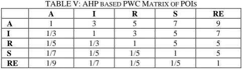
important than all three other POIs used in the study. Same study in its third weighting criteria has assigned 30% weights to A & I and 20% to S & R meaning that „I‟ is another POI which is more important than other two (R & S) and equally important to accuracy. Besides decision maker can, based on the information about the type of hardware used by an organization, type of distributive computing model used (i.e. in-house or clouding), type of dataset and focus of the study, decide about the PWC ratios for speed versus robustness. Table V shows our PWC matrix for various POIs.
TABLEV:AHP BASED PWCMATRIX OF POIS
A I R S RE
A 1 3 5 7 9
I 1/3 1 3 5 7
R 1/5 1/3 1 5 5
S 1/7 1/5 1/5 1 5
RE 1/9 1/7 1/5 1/5 1
We will use principal right eigenvector method (EM) as in [15] to solve AHP matrix. EM involves the determination of weight vector (W) from the PWC matrix (Table V) by solving the characteristic equation AW = λmaxW; where λmax
is the maximum eigen-value of A (=PWC Matrix). Three issues surround the use of the AHP [16]. The first issue is inconsistency problem and it occurs because the allowable upper bound of consistency index (CI) is 10% of the random inconsistency (RI). Consistency in PWC Matrix can be checked by the consistency ratio (CR) which is equal to {[(λmax - 1)/(n-1)]/RI}. Here RI‟s value varies with the order
of PWC matrix. A CR of less than or equal to 10% is considered of an acceptable consistency. The second issue is rank-reversal problem [18] of range of wij, the relative weight of alternative i to j. There are total of 20 alternatives (Classifier-IVSO pairs) in our case.
Third issue is discriminating-sensitivity problem i.e. if the range of wij were to be too reduced, and then CI would converge to 0, making it impossible for the AHP to discriminate an important alternative from others. This can be avoided by using Saaty‟s1-9 scale for PWCs. Our calculated CR (=CI/index of consistency) is10%. In short, our comparisons are consistent and there is no question of discriminating - sensitivity problem as well.
The objective of AHP is to compare decision alternatives (i.e. 20 Classifier-IVSO pairs) with respect to each POI and to determine the relative composite priorities for the true total weights of Classifier-IVSO pairs, when the POIs are assembled together. Our solution to our pair wise matrix gives us weights for various POI as: 0.498531 for A, 0.256196 for I, 0.148403 for R, 0.066924 for S and 0.029945 for RE. But as POIs have different dimensions or UOM, there is a problem of incommensurability. We can address the issue of differences in dimensions through normalization.
and 10 points respectively (as shown in Table VI). The intermediate intervals have equal width, which implies that essentially they are assuming a linear relationship.
TABLEVI:RULES FOR POISCORES FOR SWUF OF REF.[12]
Scores (below)
A I R S RE
0 If < 0.65 Null=1 If > 0.19
If > 100
If < 50
2 If
0.65-0.68 Null
=1
If 0.16 - 0.19
If 25 - 100
If 50 - 51
4 If
0.69-0.72 Poor=
2
If 0.12 - 0.15
If 19 - 24
If 52 - 53
6 If
0.73-0.76
Poor = 2
If 0.08 - 0.11
If 12 - 18
If 54 - 55
8 If
0.77-0.80 Mediu
m = 3
If 0.04 - 0.07
If 6 - 11
If 56 - 57
10 If > 0.80 High = 4
If < 0.04
If < 6 If > 57
Notes:
(1). Entry “50-51” means that if values of this POI vary from 50 to 51 for RE, then its score will be 2.
(2). [Poor = 2] will get score of 6 if both components are linear in the classifier-IVOR pair and [Poor=2] will get score of 4 if one of the components is linear and another nonlinear in the classifier-IVOR pair (3) [Null = 1] will get score of 2 if both components are linear in the classifier-IVOR pair and [Null = 1] will get score of 0 if one of the components is linear and another nonlinear in the classifier-IVOR pair.
General considerations for our POI can be described as follow. For accuracy (AUC test), larger value is considered better than smaller value. Similar is the case for two other POI, interpretability, and residual efficiency. On the other hand for robustness and speed, lower value is better than higher one. Individual parameters results of Tables II, III & IV has been normalized with SWUF of ref. [12] for various pairs of Classifiers-IVSO for all five POI (A, I, R, S and RE) and presented in Tables VII, VIII, IX and 10. The explanation of these three tables can be seen in study [4] and if some cell(s) has got zero value in all three tables, it has been replaced with a value of 0.0001, so as to avoid making the weight of respective POI zero. And this small adjustment had no affect on relative weights of POIs.
TABLEVII:INDIVIDUAL PARAMETERS RESULTS (NORMALIZED WITH
SWUF) OF VARIOUS PAIRS OF CLASSIFIERS-IVSO FOR ROBUSTNESS AND
INTERPRETABILITY
Robustness Interpretability
OV AV PC SV OV AV PC SV
LR 8 8 8 6 8 8 2 0
DT 8 10 8 8 10 10 2 0
NN 10 10 10 8 4 4 0 0
AB 2 2 4 0 4 4 0 0
RF 10 10 10 0 4 4 0 0
TABLEVIII:INDIVIDUAL PARAMETERS RESULTS (NORMALIZED WITH
SWUF) OF VARIOUS PAIRS OF CLASSIFIERS-IVSO FOR ACCURACY AND
SPEED POIS
Accuracy (AUC Test) Speed (Minutes)
OV AV PC SV OV AV PC SV
LR 8 8 8 8 6 4 10 0
DT 8 8 2 8 10 10 10 0
NN 8 8 0 8 10 10 10 0
AB 6 8 2 0 6 4 8 0
RF 8 1 2 0 8 2 6 0
TABLEIX:INDIVIDUAL PARAMETERS RESULTS (NORMALIZED WITH SWUF)
OF VARIOUS PAIRS OF CLASSIFIERS-IVSO FOR RESIDUAL EFFICIENCY (RE)
OP1-OV OP2-AV OP3-PCA OP2-SV
LR 4 2 4 6
DT 6 4 6 8
NN 2 0 2 4
AB 6 6 6 8
RF 8 6 8 10
TABLEX:FINAL ECIVALUES FOR AHPWEIGHTING AND
NORMALIZATIONS WITH SWUF(IN %)
OV AV PC SV
LR 8.175% 8.001% 6.008% 4.464%
DT 9.267% 9.422% 3.320% 4.733%
NN 6.964% 6.907% 1.704% 4.620%
AB 5.079% 5.876% 1.978% 0.226%
RF 7.016% 3.406% 2.553% 0.283%
TABLEXIA:ECIVALUES FOR THE DIFFERENT NM AND WC FOR OV
LR DT NN AB RF
ECImm&1 0.326 0.383 0.269 0.039 0.230
ECImm&2 0.402 0.434 0.347 0.135 0.311
ECImm&3 0.423 0.488 0.341 0.149 0.308
ECIz&1 0.551 0.667 0.388 -0.356 0.291
ECIz&2 0.565 0.599 0.406 -0.288 0.314
ECIz&3 0.587 0.717 0.351 -0.277 0.268
SWUF&AHP 0.0817 0.0927 0.0696 0.0508 0.0702
TABLEXIB:ECIVALUES FOR THE DIFFERENT NM AND WC FOR AV
LR DT NN AB RF
ECImm&1 0.307 0.417 0.241 0.023 0.238
ECImm&2 0.384 0.472 0.311 0.121 0.325
ECImm&3 0.407 0.521 0.308 0.136 0.320
ECIz&1 0.490 0.786 0.281 -0.404 0.331
ECIz&2 0.507 0.733 0.263 -0.329 0.376
ECIz&3 0.535 0.837 0.224 -0.314 0.322
SWUF&AHP 0.0800 0.0942 0.0691 0.0588 0.0341
TABLEXIC:ECIVALUES FOR THE DIFFERENT NM AND WC FOR PC
LR DT NN AB RF
ECImm&1 0.168 0.006 -.042 -0.076 0.102
ECImm&2 0.259 0.053 -0.037 0.014 0.146
ECImm&3 0.227 0.045 -0.033 0.007 0.129
ECIz&1 0.098 -0.518 -0.744 -0.725 -0.191
ECIz&2 0.151 -0.638 -1.025 -0.691 -0.315
ECIz&3 0.025 -0.673 -1.011 -0.731 -0.382
SWUF&AHP 0.0601 0.0332 0.0170 0.0198 0.0255
TABLEXID:ECIVALUES FOR THE DIFFERENT NM AND WC FOR SV
LR DT NN AB RF
ECImm&1 -0.143 -0.129 -0.057 - -
ECImm&2 -0.019 -0.006 0.070 - -
ECImm&3 -0.025 -0.014 0.054 - -
ECIz&1 -0.970 -0.739 -0.490 - -
ECIz&2 -0.891 -0.600 -0.330 - -
ECIz&3 -0.914 -0.656 -0.415 - -
SWUF&AHP 0.0446 0.0473 0.0462 0.0023 0.0028
The results (in Tables XI A-XI D) have shown that our method has proven to be robust on following grounds. First of all it has not generated any negative entries. Secondly, contrary to the results from study [4] which have kept almost the same hierarchy for all classifiers with only few minor exceptions, results of this study has not followed any specific pattern regarding ranking for all classifiers as our results has provided a different ranking of DM classifiers for all four different types of input variables. And this is important because performance of data mining models is dependent on factors like problem in hand, type of dataset, depth of database, types and nature of relationships among input
variables and/or target variables. Thus ranking of DM models should not be considered permanent and should change as these factors change. This is, however, different from objective ranking drawn for various DM models from the broader categories of inputs used, as has been attempted here. Last but not least, our method was able to rank all the classifiers for all variable types as opposed to study [4] who was not able to rank AB and RF for VS.
In short, the new methodology using AHP as weighting the assessment criteria or POI and with SWUF as normalization technique to tackle the issue of incommensurability because of difference in UOM for POI (or criteria) has worked well in ranking data mining algorithms. Another main contribution of the paper was the development of a fifth POI (named as RE) from ten characteristics of interest (COI) derived from vast body of data mining literature, have worked very well in ranking the data mining algorithms and the robustness of our results are deeply indebted to this fifth POI.
REFERENCES
[1] S. Anjum, “Early warning system for financial crisis: a critical review and application of data mining approach,” Ph. D. Dissertation, GSID, Nagoya University, Japan, March 2003.
[2] L. C. Tjung, O. Kwon, K. C. Tseng, and J. Bradley, “Forecasting financial stocks using data mining,” Craig School of Business, CSU, Fresno, 2010.
[3] A. Nadali, S. Pourdarab, and H. E. Nosratabadi, “Labeling the class of bank credit‟s customers by a fuzzy expert system for credit scoring with data mining approach,” in Proc. IEEE Knowledge Discovery Conference, 2011.
[4] M. Clemente, V. G. Bosch, and S. San Matías. (2010). Assessing classification methods for churn prediction by composite indicators. Manuscript. Dept. of Applied Statistics and Quality. Universitat Politècnica de València. Camino de Vera s/n. 46022 Spain. [Online]. Available:
http://www.upv.es/deioac/Investigacion/ManuscriptDSS.pdf [5] B. Kramer, D. Kronbichler, T. V. Welie,and J. Putman, “Comparing
social objectives for decision-making in housing corporations,” Applied Working Paper, no. 2008-02, Ortec Finance Research Center (OFRC) working paper series, May 2008, Rotterdam.
[6] K. McGarry, “A survey of interestingness measures for knowledge discovery,” The Knowledge Engineering Review, Cambridge University Press, pp. 1–24, 2005.
[7] R. Gerritsen, “Assessing loan risks: a data mining case study,” IT Pro, IEEE,November/December, 1999.
[8] K. Niki and H. R. Weistroffer, “Expanding the knowledge base for more effective data mining,” Manuscript, Virginia Commonwealth University, 1015 Floyd Avenue, School of Business, P. O. Box 844000-4000, Richmond VA, USA, 2005.
[9] J. Thongkam, G. Xu, and Y. Zhang, “AdaBoost algorithm with random forests for predicting breastcancer survivability,” in Proc. Intl. Joint Conf. on Neural Networks (IJCNN 2008), IEEE, 2008.
[10] T. Hastie, R. Tibshirani, and J. Friedman, The elements of statistical learning: Data mining, inference, and prediction, Springer Series in Statistics, 2nd ed., 2008.
[11] SAS, Data mining using as enterprise miner: A case study approach, SAS Publishing, 2003.
[12] Hemphill, L. J. Berry, and S. McGreal, “An indicator-based approach to measuring sustainable urban regeneration performance: Conceptual foundations and methodological framework,” Urban Studies,vol.414, ch. 1, pp. 725-755, 2004.
[13] T. L. Saaty, The Analytic Hierarchy Process, Mc Graw-Hill, NY, 1980. [14] K. Al-Harbi and M. Al-Subhi, “Application of the AHP in project management,” Intl. Journal of Project Management, vol. 19, pp. 19-27, 2001.
[15] S. I. Gass and T. Rapcsak, “Singular value decomposition in AHP,” presented at International Symposium on the Analytic Hie-rarchy Process, Berne, Switzerland, August, 2001.
Shahid W. Anjum is an adjunct faculty member (Finance and MIT), a member of dissertation committee for Doctor of Management Information Technology (DMIT) program and has been teaching Financial Valuation course to Doctor of Business Administration (DBA) program at College of Management, Lawrence Technological University (LTU) in USA, besides working for one of the leading financial institutions in Canada.