Improving the ensemble transform Kalman filter using a second-order Taylor approximation of the nonlinear observation operator

www.nonlin-processes-geophys.net/21/955/2014/ doi:10.5194/npg-21-955-2014

© Author(s) 2014. CC Attribution 3.0 License.

Improving the ensemble transform Kalman filter using

a second-order Taylor approximation of the nonlinear

observation operator

G. Wu1, X. Yi1, L. Wang2, X. Liang3, S. Zhang1, X. Zhang1, and X. Zheng1

1_{State Key Laboratory of Remote Sensing Science, College of Global Change and Earth System Science,}

Beijing Normal University, Beijing, China

2_{Department of Statistics, University of Manitoba, Winnipeg, Canada}

3_{National Meteorological Information Center, China Meteorological Administration, Beijing, China}

Correspondence to: X. Zheng ([email protected])

Received: 28 January 2014 – Published in Nonlin. Processes Geophys. Discuss.: 11 April 2014 Revised: 22 July 2014 – Accepted: 8 August 2014 – Published: 23 September 2014

Abstract. The ensemble transform Kalman filter (ETKF) as-similation scheme has recently seen rapid development and wide application. As a specific implementation of the ensem-ble Kalman filter (EnKF), the ETKF is computationally more efficient than the conventional EnKF. However, the current implementation of the ETKF still has some limitations when the observation operator is strongly nonlinear. One problem in the minimization of a nonlinear objective function similar to 4D-Var is that the nonlinear operator and its tangent-linear operator have to be calculated iteratively if the Hessian is not preconditioned or if the Hessian has to be calculated sev-eral times. This may be computationally expensive. Another problem is that it uses the tangent-linear approximation of the observation operator to estimate the multiplicative inflation factor of the forecast errors, which may not be sufficiently accurate.

This study attempts to solve these problems. First, we ap-ply the second-order Taylor approximation to the nonlin-ear observation operator in which the operator, its tangent-linear operator and Hessian are calculated only once. The related computational cost is also discussed. Second, we propose a scheme to estimate the inflation factor when the observation operator is strongly nonlinear. Experimentation with the Lorenz 96 model shows that using the second-order Taylor approximation of the nonlinear observation op-erator leads to a reduction in the analysis error compared with the traditional linear approximation method. Further-more, the proposed inflation scheme leads to a reduction

in the analysis error compared with the procedure using the traditional inflation scheme.

1 Introduction

The spatial and temporal distribution of observations is con-tinuously changing with the improvement in numerical mod-els and observation techniques. Sounding data, remote sens-ing observations, satellite radiance data and other indirect information bring both opportunities and challenges in data assimilation. How to assimilate these indirect observations is an important research topic in data assimilation (Re-ichle, 2008).

The observation operators for indirect observations are of-ten nonlinear. For example, radiative transfer codes (e.g., RT-TOV, CRTM, Saunders et al., 1999; Han et al., 2006) can be treated as observation operators by mapping air temper-ature and moisture to the microwave radio brightness tem-perature (McNally, 2009). Because the relationship of these observations with modeled variables may be strongly nonlin-ear (Liou, 2002) and the observation errors may be spatially correlated (Miyoshi et al., 2013), data assimilation schemes have to be appropriately designed to address such indirect observations.

variational data assimilation schemes (VAR; e.g., Parrish and Derber, 1992; Courtier et al., 1994; Lorenc, 2003) can assim-ilate data with nonlinear observation operators and spatially correlated observation errors. However, a drawback of VAR is that it has to calculate the adjoint of a dynamical model, which is not an easy task in practice. Moreover, VAR does not give a direct estimate of the background error covari-ance matrix, which is crucial for the performcovari-ance of any data assimilation scheme. In general ensemble data assimilation, the maximum likelihood ensemble filter (MLEF) minimizes a cost function that depends on a general nonlinear observa-tion operator to estimate the state vector, which is equivalent to maximizing the likelihood of the posterior probability dis-tribution (Zupanski, 2005). The particle filter uses a set of weighted random samples (particles) to approximate the pos-terior probability distribution that may depend on a nonlinear observation operator (van Leeuwen, 2009).

The ensemble Kalman filter (EnKF) scheme has a strategy to optimize forecast error statistics without using the adjoint of the dynamical model (e.g., Evensen, 1994a, b; Burgers et al., 1998; Anderson and Anderson, 1999; Wang and Bishop, 2003; Wu et al., 2013). It is also conceptually applicable to data assimilation with nonlinear observation operators. How-ever, it has been demonstrated that when the observation op-erator is strongly nonlinear, using the linear approximation of the observation operator to derive the error covariance evo-lution equation can result in an oversimplified closure and dubious performance of the EnKF (e.g., Miller et al., 1994; Evensen, 1997; Yang et al., 2012).

The ensemble transform Kalman filter (ETKF) was first introduced in atmospheric assimilation by Bishop and Toth (1999) and Bishop et al. (2001). Wang and Bishop (2003) transformed the forecast perturbations into analysis perturbations by multiplying a transformation matrix. They also proposed an efficient way to construct the transform ma-trix through eigenvector decomposition of a mama-trix of the en-semble size. Hunt et al. (2007) extended the ETKF method to deal with a general nonlinear observation operator using the cost function. In addition to the reduction of computational cost compared with EnKF, another advantage of the ETKF proposed by Hunt et al. (2007) is that it can assimilate obser-vations with strongly nonlinear observation operators (Chen et al., 2009) and with spatially correlated observation errors (Stewart et al., 2013).

However, there are still problems associated with the ETKF when the observation operator is strongly nonlinear. First, the current ETKF is based on the minimization of a cost function similar to that in VAR for nonlinear observation op-erators (Hunt et al., 2007). First, the direct calculation for the minima requires iterative evaluation of the nonlinear opera-tors and their tangent-linear operaopera-tors. Using linear approx-imation of the nonlinear observation operators (e.g., Hunt et al., 2007) can effectively reduce the computational burden, but at the cost of increasing analysis error. Second, tangent-linear approximation of the observation operator is used for

the forecast error inflation in the ETKF (e.g., Li et al., 2009). If the observation operators are strongly nonlinear, the in-flation factors and hence the forecast error covariance ma-trices may be estimated erroneously, leading to an eventual increase in the analysis error.

In this study, we propose two alternative approaches to im-proving assimilation quality when the observation operator is strongly nonlinear. First, in an effort to reduce computa-tional cost without significantly reducing estimation quality, we use the second-order Taylor expansion of the observation operator to estimate both the inflation factors and the ana-lysis states. Second, for the case where the inflation factor is constant in space, we propose a new forecast error inflation method for general nonlinear observation operators without using tangent-linear approximation. It is worthwhile pointing out that the proposed methodology implicitly assumes the use of incremental minimization with outer and inner loops. There may be other efficient methods available in mathemat-ical optimization and control theory.

The potential use of the second-order information has been noted by some authors. For example, Hunt et al. (2007) noted that the second-order derivatives of the objective function might be used to estimate the covariance of analysis weight, which is an important step in ETKF with a nonlinear observa-tion operator. Moreover, Le Dimet et al. (2002) and Daescu and Navon (2007) noted that the second-order information in nonlinear variational data assimilation is important to the issue of solution uniqueness.

In the conventional ETKF scheme, linear approximation of nonlinear observation operators is used for the purpose of reducing the computational cost compared with conven-tional methods of searching for the minima of nonlinear cost functions (Hunt et al., 2007). This study also aims to inves-tigate the changes in analysis errors when a nonlinear obser-vation operator is substituted by its first-order and second-order Taylor approximations. However, we focus on the for-mulation of the forecast error inflation method in the case of a nonlinear observation operator, and on the improved accuracy with second-order versus first-order approximation or linear approximation. Further studies on the performance of the proposed schemes in practical data assimilations are needed, and should be performed in the future.

The rest of the paper is organized as follows. Our modified ETKF schemes are described in Sect. 2. The assimilation re-sults in a Lorenz 96 model with a nonlinear observation sys-tem are presented in Sect. 3. The discussions are given in Sect. 4, and the conclusions are in Sect. 5.

2 Methodology

2.1 ETKF with forecast error inflation

procedures for forecast error inflation. In this section, we pro-pose an inflation scheme for general nonlinear observation operators.

Using the notations of Ide et al. (1997), a nonlinear discrete-time forecast and observation system can be written as

xt_i=Mi−1 xa_i−1

+ηi, (1)

yo_i =Hi xti

+εi, (2)

where i is the time step index; xt_i=

n

x₁t_,i, x₂t_,i, . . . , x_n,it

oT

is the n-dimensional true state vector; xa_i−1=

n

x₁a_,i−1, x₂a_,i−1, . . . , x_n,ia ₋₁oT is the n-dimensional analysis state vector that is an estimate ofxt_i−1;Mi is the nonlinear forecast operator; yo_i =ny₁o_,i, y₂o_,i, . . . , y_pi,io oT is the pi -dimensional observation vector;Hi=h1,i, h2,i. . . , hpi,i

T

is the nonlinear observation operator, where hk,i is an n-dimensional multivariate function; andηi andεi are the forecast and observation error vectors that are assumed to be statistically independent of each other, time uncorrelated, and to have mean zero and covariance matrices Pi and Ri, respectively. The detailed procedure of the ETKF with a nonlinear observation operator (Hunt et al., 2007) with the proposed inflation scheme is as follows.

Step 1. Calculate thejth perturbed forecast state at timei as

xf_i,j =Mi−1

xa_i−1,j, (3)

wherexa_i−1,j is thejth perturbed analysis state at timei−1. Then, the mean forecast state is defined as

xf_i = 1 m

m

X

j=1

xf_i,j, (4)

wheremis the total number of ensemble members.

Step 2. Assume the forecast errors to be in the form √

λi

xf_i,j−xf_i, j =1,2, . . . , m, where the inflation fac-torλi can be estimated by minimizing the objective function

Li(λ)=Tr

h

didTi −Ci(λ)−I didTi −Ci(λ)−I

Ti

. (5)

Here, I is thepi×pi identity matrix,

di =R−1_i /2

yo_i −Hi

xf_i (6)

is the innovation vector normalized by the square root of the observation error covariance matrix (Wang and Bishop,

2003), and

Ci(λ)≡ 1 m−1

m

X

j=1

h

R−1_i /2Hi

xf_i+ √

λxf_i,j−xf_i

−Hi

xf_i Hi

xf_i+ √

λxf_i,j−xf_i

−Hi

xf_iTR−1_i /2i. (7)

(See Appendix A for details.)

Step 3. Calculate the analysis state as

xa_i =xf_i+

q

ˆ λiXfiw

a

i, (8)

where

Xf_i =xf_i,1−xf_i,x_i,f₂−xf_i, . . . ,xf_i,m−xf_i (9) andwa_i is estimated by minimizing the objective function

Ji(w)= 1

2(m−1)w T_w+1

2

h

yo_i −Hi

xf_i+

q

ˆ λiXfiw

iT

R−1_i hyo_i −Hi

xf_i+

q

ˆ λiXfiw

i

. (10)

Step 4. Calculate a perturbed analysis state as

xa_i,j=xa_i+

q

ˆ λiXfiW

a

i,j, (11)

where Wa_i,j is the jth column of the matrix Wa_i = √

m−1_J¨ i|wa_i

−1/2

and _J¨

i|wa_i is the second-order

deriva-tive ofJi(w)atwa_i (see Appendix B for details). Lastly, set i=i+1 and return to Step 1 for the next iteration.

To estimate the inflation factor, Li et al. (2009) proposed a scheme that requires the tangent-linear operator of the ob-servation operator (see Sect. 2.2.1 for the definition). In an effort to reduce the computational cost of searching for the minima of the objective function (Eq. 10), Hunt et al. (2007) suggested the following linear approximation:

Hi

xf_i+

q

ˆ λiXfiw

≈Hi

xf_i+Yf_iw, (12)

where Yf_i =nHi

q

ˆ λi

xf_i,1−xf_i+xf_i−Hi

xf_i,

Hi

q

ˆ λi

xf_i,2−xf_i+xf_i−Hi

xf_i, . . . ,

Hi

q

ˆ λi

xf_i,m−xf_i+xf_i−Hi

xf_i o. (13)

2.2 Simplified estimation methods in special cases To compute the variational minimization in Eq. (10) op-erationally, one can directly compute the explicit solution of the minima and iterate the process as in the 4D-Var outer loop (Lorenc, 2003; Liu et al., 2008). However, do-ing so still requires repeatedly calculatdo-ing the nonlinear func-tionHi

xf_i+

q

ˆ λiXf_iw

and its tangent-linear operator (see Sect. 2.2.1 for the definition), which depend on w andxf_i. In this subsection, we propose an alternative procedure when the observation operatorHi can be approximated by its Tay-lor expansions.

2.2.1 First-order Taylor approximation forHi

The first-order Taylor approximation for Hi at the forecast state vectorxf_i is defined as

Hi xti

≈Hi

xf_i+ ˙H_i|xf

i

xt_i−xf_i, (14)

where

˙ H_i|xf

i =    

∂h1,i ∂x1,i

· · · ∂h1,i ∂xn,i ..

. . .. ... ∂h_{pi ,i}

∂x1,i · · · ∂h_{pi ,i}

∂xn,i    

xi=xfi

(15)

is the first-order derivative of Hi evaluated at the forecast statexf_i (tangent-linear operator). Then,λi can be estimated by minimizing the quadratic function

L1,i(λ)=Tr

h

didTi −λR

−1/2

i H˙i|xf

i ˆ PiH˙

T i|xf

iR

−1/2

i −I

didTi −λR

−1/2

i H˙i|xf

i ˆ PiH˙

T i|xf

iR

−1/2

i −I

Ti

. (16) The analytic solution is

ˆ λi=

TrhR−1_i /2H˙_i|xf

i ˆ PiH˙

T i|xf_iR

−1/2

i didTi −I

Ti

TrhR−1_i /2H˙_i|xf

i ˆ PiH˙

T i|xf

iR

−1

i H˙i|xf

i ˆ PiH˙

T i|xf

iR

−1/2

i

i, (17)

where ˆ Pi=

1 m−1X

f

i

Xf_iT. (18)

Similarly,wa_i can be estimated by minimizing the multivari-ate quadratic function

J1,i(w)= 1

2(m−1)w T_w

+1 2

h

yo_i −Hi

xf_i−

q

ˆ λiH˙_i|xf

iX

f

iw

iT

R−1_i hyo_i −Hi

xf_i−

q

ˆ λiH˙i|xf

iX

f

iw

i

, (19)

and the analytic solution is

wa_i =

(m−1)I+ ˆλX_ifTH˙T_i|xf

iR

−1

i H˙i|xf

iX f i −1 q ˆ λi

Xf_i T

˙ HT_i|xf_iR−1i

yo_i −Hi

xf_i. (20)

(See Appendix C for details.)

2.2.2 Second-order Taylor approximation forHi

The second-order Taylor approximation forHi atxf_i is de-fined as

Hi(xti)≈Hi

xf_i+ ˙H_i|xf

i

xt_i−xf_i+1 2

xt_i−xf_iT

⊗ ¨H i|xf_i ⊗

xt_i−xf_i, (21)

whereH˙_i|xf

iis the tangent-linear operator defined in Eq. (15), and H¨_i|xf

i

≡nH¨_1,i|xf

i, . . . , ¨ H_p

i,i|xfi

oT

is the second-order derivative ofHi atxf_i, which is api-dimensional vector with thekth element meaning the following Hessian matrix:

¨

H_k,i|xf i ≡     

∂2_h k,i

∂x1,i∂x1,i · · ·

∂2_h k,i

∂x1,i∂xn,i

. .

. . .. ... ∂2hk,i

∂xn,i∂x1,i · · ·

∂2hk,i

∂xn,i∂xn,i     

xi=xf_i

k=1, . . . , pi. (22)

Here,⊗is the outer product operator; i.e., for two arbitrary n-dimensional vectorsxandy,

xT⊗ ¨H_i|xf

i ⊗y=

n

xTH_1,i|xf

iy, . . . ,x T_H¨

pi,i|xf

iy

oT

, (23) is api-dimensional vector. Then,λican be estimated by min-imizing the polynomial objective function ofλ1/2

L2,i(λ)=Tr

h

didTi −λR

−1/2

i H˙i|xf

i ˆ PiH˙

T i|xf

iR

−1/2

i

−λ3/2C1,i−λ3/2CT1,i−λ

2_C 2,i−I

didTi −λR

−1/2

i H˙i|xf_iPˆiH˙ T i|xf

iR

−1/2

i −λ

3/2_C 1,i

−λ3/2CT_1,i−λ2C2,i−I

Ti

, (24)

where

C1,i= 1 2(m−1)

m

X

j=1

h

R−1_i /2H˙_i|xf

i

p

λi

xf_i,j−xf_i xf_i,j−xf_iT⊗ ¨H_i|xf

and C2,i=

1 4(m−1)

m

X

j=1

h

R−1_i /2xf_i,j−xf_iT ⊗ ¨H_i|xf

i ⊗xf_i,j−xf_ix_i,jf −xf_iT⊗ ¨H_i|xf

i

⊗xf_i,j−xf_iTR−1_i /2i (26) are twom×mmatrices.

Moreover,wa_i can be estimated by minimizing the multi-variate polynomial objective function

J2,i(w)≈ 1

2(m−1)w T_w+1

2

h

yo_i−Hi

xf_i−

q

ˆ λiH˙_i|xf

iX f iw

− ˆ λi

2

Xf_iwT⊗ ¨H_i|xf

i

⊗Xf_iw

iT

R−1_i

h

yo_i −Hi

xf_i−

q

ˆ λiH˙_i|xf

iX

f

iw− ˆ λi

2

Xf_iwT

⊗ ¨H_i|xf

i

⊗Xf_iwi (27)

(see Appendix D for details). 2.3 Validation statistics

In the following experiments, the “true” statext_i is known by experimental design, and is non-dimensional. In this case, we can use the root mean square error of the analysis state (A-RMSE) to evaluate the accuracy of the assimilation results. The A-RMSE at theith step is defined as

A-RMSE=

r

1 n

xa_i−xt_i

2

, (28)

wherek·kdenotes the Euclidean norm, andnis the dimen-sion of the state vector. A smaller A-RMSE indicates a better performance of the assimilation scheme.

Following Anderson (2007) and Liang et al. (2012), the root mean square error of the forecast state (F-RMSE) and the spread of the forecast state (F-Spread) at theith step are defined as

F-RMSE=

r

1 n

xf_i−xt_i

2

(29) and

F-Spread=

v u u t

1 n(m−1)

m

X

j=1

x

f

i,j−xfi

2

. (30)

Roughly speaking, ifxf_i,j andxt_i are identically distributed with a mean value ofxf_i, then F-RMSE and F-Spread should be consistent with each other. This is more likely the case if the model error is small. In general, the F-RMSE can be decomposed into an F-Spread component and a model error

component, so it is larger than F-Spread (see Appendix B of Wu et al., 2013, for a detailed proof). Besides model error, the nonlinearities and the sampling error may also affect the consistency between F-RMSE and F-Spread, as is discussed later in this paper.

3 Experiments with the Lorenz 96 model

In Sect. 2.1, we outlined the general ETKF assimilation scheme with second-order least squares (SLS) error covari-ance matrix inflation. In Sect. 2.2, we proposed simplified estimation methods for two special cases whereHi either is tangent linear (Sect. 2.2.1) or can be approximated by the second-order Taylor expansion (Sect. 2.2.2). In this section, we apply these assimilation schemes to the Lorenz 96 model (Lorenz, 1996) with model errors and a nonlinear observa-tion system, because it is a nonlinear dynamical system with properties relevant to realistic forecast problems.

3.1 Description of the dynamic and observation system The Lorenz 96 model (Lorenz, 1996) is a strongly nonlinear dynamical system with quadratic nonlinearity governed by the equation

dXk

dt =(Xk+1−Xk−2) Xk−1−Xk+F, (31) wherek=1,2, . . . , K (K=40, so there are 40 variables). We apply the cyclic boundary conditions X−1=XK−1, X0=XK, andXK+1=X1. The dynamics of Eq. (31) are

“atmosphere-like” in that the three terms on the right-hand side consist of a nonlinear advection-like term, a damping term and an external forcing term, respectively. These terms can be thought of as a given atmospheric quantity (e.g., zonal wind speed) distributed on a latitude circle.

We solve Eq. (31) using the fourth-order Runge–Kutta time integration scheme (Butcher, 2003), with a time step of 0.05 non-dimensional units to derive the true state. This is equivalent to about 6 h in real time, assuming that the characteristic timescale of the dissipation in the atmosphere is 5 days (Lorenz, 1996). In our assimilation schemes, we set F =8 so that the leading Lyapunov exponent implies an error-doubling time of approximately 8 time steps (i.e., 0.4 non-dimensional time units), and the fractal dimension of the attractor is 27.1 (Lorenz and Emanuel, 1998). The initial condition is chosen to be Xk=F when k6=20 and X20=1.001F.

Because the microwave brightness temperature is an expo-nential function of soil temperature, we use the expoexpo-nential observation function to mimic the radiative transfer model in this study. Suppose the synthetic observation generated at the kth model grid point is

where k=1, . . . , pi, and εi=ε1,i,ε2,i, . . . ,εpi,i T

is the observation error vector with mean zero and covariance ma-trix Ri. Here,αis a parameter controlling the nonlinearity of the observation operator, andα=0 corresponds to the lin-ear case. All 40 model variables are observed in our exper-iments. Suppose the observation errors are spatially corre-lated. The leading-diagonal elements of Ri areσo2=1, and

the off-diagonal elements at site pair (j,k) are Ri(j, k)=σo2·0.5min(

|j−k|,40−|j−k|)_{. (33)} With the exponential observation function and spatially cor-related observation errors, the proposed scheme may poten-tially be applied to assimilate remote sensing observations and radiance data.

We added model errors to the Lorenz 96 model because they are inevitable in real dynamic systems. The model is a forced dissipative model with a parameterF that controls the strength of the forcing (Eq. 31). It behaves quite differently with different values ofF, and it produces chaotic systems with integer values ofF larger than 3. Thus, we used various values ofF to simulate a wide range of model errors while retainingF =8 when generating the “true” state. These ob-servations were then assimilated with F =4,5, . . . ,12. We simulated observations every 4 time steps for 100 000 steps to ensure robust results (Sakov and Oke, 2008; Oke et al., 2009). The ensemble size is 30.

3.2 Assimilation results

In this section, we examine the following five data assimi-lation methods corresponding to five different treatments of nonlinearity in inflation factor estimation and optimization:

ETKF: traditional ETKF in linear approximation (Eq. 12) and optimization (Eq. 10).

TT: tangent-linear approximation in both inflation (Eq. 17) and optimization (Eq. 20).

TN: tangent-linear approximation in inflation (Eq. 17) and nonlinearity in optimization (Eq. 10).

SS: second-order approximation in both inflation (Eq. 24) and optimization (Eq. 27).

NN: nonlinearity in both inflation (Eq. 5) and optimiza-tion (Eq. 10).

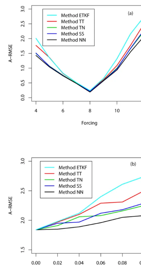
The corresponding time-mean A-RMSEs of these as-similation schemes withα=0.1 andF =4,5, . . . ,12, over 100 000 time steps, are plotted in Fig. 1a. First, the figure clearly shows that for each estimation method, the A-RMSE increases as F becomes increasingly distant from the true value of 8.

Moreover, method NN has a smaller A-RMSE uniformly over all values ofF than method TN, indicating that the pro-posed nonlinear inflation estimation (Eq. 5) performs bet-ter than the tangent-linear inflation scheme (Eq. 17). On

Figure 1. (a) Time-mean values of the A-RMSE as a function of

forcingFfor different assimilation methods in the Lorenz 96 model

and the observation operator (Eq. 32) with parameter α=0.1.

(b) Time-mean values of the A-RMSE as a function of parameter

αfor different assimilation methods in the Lorenz 96 model with

F=12. ETKF: traditional ETKF in linear approximation (Eq. 12)

and optimization (Eq. 10) (cyan line); TT: tangent-linear approx-imation in both inflation (Eq. 17) and optimization (Eq. 20) (red line); TN: tangent-linear approximation in inflation (Eq. 17) and nonlinearity in optimization (Eq. 10) (green line); SS: second-order Taylor approximation in both inflation (Eq. 24) and optimization (Eq. 27) (blue line); NN: nonlinearity in both inflation (Eq. 5) and optimization (Eq. 10) (black line). The ensemble size is 30.

the partial nonlinear method and is better than the first-order Taylor approximation method. Lastly, the traditional ETKF method has the largest A-RMSE, which implies that although the linear approximation is computationally more efficient, it may introduce a larger analysis error.

For the Lorenz 96 model with a large error (F =12), the time-mean A-RMSEs and F-RMSEs of the five methods are given in Table 1, as well as the time-mean values of the ob-jective functions. The function represents the second-order distance from the squared innovation statistic (didTi ) to its expectation. Generally speaking, for a more accurate assim-ilation scheme, the realization of d_idT

i should be closer to its expectation, and therefore the value of the objective func-tion should be smaller. It can be seen that the full nonlinear method (NN) has both the smallest A-RMSE and F-RMSE, while the traditional linear approximation method (ETKF) has the largest RMSEs. The second-order Taylor approxima-tion method (SS) performs similarly to the partial nonlinear method (TN), but better than the first-order Taylor approxi-mation method (TT). In the majority of the cases, a smaller error corresponds to a smaller value of the objective func-tionL. The ratios of F-RMSEs to A-RMSEs are also listed in Table 1, which can be considered a measurement of the improvement gained at the analysis step. All the ratios are larger than 1, which indicates that the analysis state is bet-ter than the forecast state. Among all methods, the ratio is largest for the TN method, which indicates the largest error reduction at the analysis step.

To illustrate the variation in A-RMSE with respect to the parameter α, the corresponding time-mean A-RMSEs of different assimilation schemes with F =12 and α= 0,0.02,0.04,0.06,0.08,0.1 are plotted in Fig. 1b. It shows that all the schemes have the same A-RMSE withα=0 (i.e., the observation operator is linear), indicating that there is no difference between them. For each scheme, the A-RMSE in-creases as the parameterαincreases from 0 to 0.1. The mag-nitude relation of all schemes is basically consistent with that in Fig. 1a. The larger the parameterαis, the bigger the dif-ference that the different schemes have.

To investigate the consistency between RMSE and F-Spread, we present the time-mean values of the five meth-ods for casesF =12 andF =8 in Tables 2 and 3, respec-tively, as well as the ratios of F-RMSE to F-Spread. It is easy to see that in all cases, the RMSEs are larger than the F-Spreads, and therefore, all the ratios are greater than 1. How-ever, the ratio of the full nonlinear method (NN) is the small-est, while the ratio of the linear approximation method is the largest. The ratio of the second-order approximation method (SS) is comparable to that of the partial nonlinear method (TN), but smaller than that of the first-order approxima-tion method (TT). This suggests that the ensemble-perturbed predictions are the most (least) reasonable for method NN (ETKF). Moreover, the ratios with F =8 are much closer to 1 than those withF =12, because the model error with F =12 is much larger than that withF =8 (see Sect. 2.3).

Table 1. The time-mean values of A-RMSE and F-RMSE, the ratio

of F-RMSE to A-RMSE, and the objective function (second-order distance from the squared innovation statistic to its expectation) in the five ETKF methods for the Lorenz 96 model, with forcing

parameterF=12 and parameter of observation operatorα=0.1.

ETKF: traditional ETKF in linear approximation (Eq. 12) and op-timization (Eq. 10); TT: tangent-linear approximation in both in-flation (Eq. 17) and optimization (Eq. 20); TN: tangent-linear ap-proximation in inflation (Eq. 17) and nonlinearity in optimization (Eq. 10); SS: second-order Taylor approximation in both inflation (Eq. 24) and optimization (Eq. 27); NN: nonlinearity in both infla-tion (Eq. 5) and optimizainfla-tion (Eq. 10).

Scheme ETKF TT TN SS NN

A-RMSE 2.74 2.50 2.25 2.29 2.08

F-RMSE 3.20 3.00 2.77 2.66 2.52

F-RMSE/

A-RMSE 1.17 1.20 1.23 1.16 1.21

L 49 700 074 17 078 480 8 768 825 9 177 962 8 458 902

Table 2. The time-mean values of F-RMSE and F-Spread, and the

ratio of F-RMSE to F-Spread in the four ETKF schemes for the

Lorenz 96 model, with forcing parameterF=12 and parameter of

observation operatorα=0.1.

Scheme ETKF TT TN SS NN

F-RMSE 3.20 3.00 2.77 2.66 2.52

F-Spread 1.06 1.45 1.46 1.48 1.45

F-RMSE/F-Spread 3.02 2.07 1.90 1.80 1.74

Table 3. Similar to Table 2, but withF=8.

Scheme ETKF TT TN SS NN

F-RMSE 0.30 0.29 0.26 0.27 0.23

F-Spread 0.20 0.22 0.21 0.22 0.21

F-RMSE/F-Spread 1.50 1.32 1.24 1.18 1.09

3.3 Impacts of Taylor approximations

In Sect. 3.2, we see that the A-RMSEs derived from the five ETKF assimilation schemes are close whenF is close to the true value of 8, but are different whenF departs from 8. This effect may depend on how well the Taylor expansions ap-proximate the nonlinear observation operatorHi.

For example, the Taylor expansion of thekth component of observation operatorHi(x)=xexp{αx}(Eq. 32) withα= 0.1 around the forecast statexf_k,iis

xt_k,iexp

0.1xt_k,i =xf_k,iexpn0.1xf_k,io+1+0.1xf_k,i

expn0.1xf_k,io xt_k,i−x_k,if +0.2+0.01xf_k,i

To verify how well the Taylor expansions approximate the nonlinear observation operatorHi, we calculate the ratios of the Taylor expansion residuals over xt_k,iexpn0.1xt_k,io. If a ratio falls outside the interval [−0.1, 0.1], then the corre-sponding residual cannot be regarded as being of a higher order infinitesimal, and hence cannot be ignored. There-fore, a larger proportion of ratios falling outside the inter-val [−0.1, 0.1] indicates a worse Taylor expansion, and vice versa.

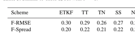
The proportions of the ratios that fall outside the inter-val [−0.1, 0.1] are plotted in Fig. 2, which shows that when F =8, the proportions are 0.0169 and 0.0006 for the first-order and second-first-order Taylor expansions, respectively. This result indicates that at almost all times and locations, both the first-order and second-order Taylor expansions are good ap-proximations ofxt_k,iexpn0.1xt_k,io. However, whenF =12, at approximately 47 % (19 %) of the times and locations,

xt_k,iexpn0.1xt_k,iocannot be approximated adequately by its first-order or second-order Taylor expansion. Therefore, the A-RMSEs derived by the five ETKF schemes are quite dif-ferent. This example also indicates that the success of the Taylor approximation method depends on both the smooth-ness ofHi and the range of forecast states. It seems that for the same strongly nonlinear observation operator, the larger the model error, the less the success of the Taylor approxi-mation.

4 Discussions 4.1 Inflation

It is widely recognized that the initial estimates of ensemble forecast errors should be inflated to improve assimilated re-sults. To date, however, all of the existing adaptive inflation schemes in ETKF are based on the assumption that the obser-vation operator is linear or tangent linear (e.g., Li et al., 2009; Miyoshi, 2011). In this study, a method to estimate the mul-tiplicative inflation factors is proposed for general nonlinear observation operators.

Historically, in systems such as the Met Office ETKF (Flowerdew and Bowler, 2011), the need for inflation arises primarily due to spurious correlations that cause the raw ana-lysis ensemble to be severely underspread even when the background ensemble is well spread. In this case, therefore, inflation must be applied to the analysis ensemble to respond correctly to the actual analysis uncertainty in the nonlin-ear forecast step. Inflation of the background ensemble may be more appropriate when the inflation primarily represents forecast model error, although stochastic physics or additive inflation may also be appropriate in this case (Hamill and Whitaker, 2005; Wu et al., 2013).

Our choice to inflate the background ensemble is crucial to the ability to find a direct nonlinear solution for Eqs. (5)–(7),

Figure 2. The proportions of residual ratios of the first-order (solid

line) and second-order (dotted line) Taylor expansions over the non-linear observation operatorxt_k,iexpn0.1xt_k,iothat fall outside the interval [−0.1, 0.1], as a function of forcingF.

because of the way the inflation factor appears in these equa-tions. The objective function for estimating the multiplica-tive inflation factors is the second-order distance between the expectations of the squared innovation and its realization, which also makes the rms spread equal to the rms error (e.g., Palmer et al., 2006; Wang and Bishop, 2003; Flowerdew and Bowler, 2011).

The proposed nonlinear method is tested using the Lorenz 96 model with nonlinear observation systems (Sect. 3.2). The resulting A-RMSEs are clearly smaller than those of the first-order Taylor approximation in the estima-tion of the inflaestima-tion factor. This indicates that the proposed full nonlinear inflation method is better than the first-order Taylor approximation inflation method in the case of non-linear observation operators (i.e., method NN is better than method TN). In addition, the F-RMSE and F-Spread of the proposed nonlinear method are more consistent than those of the first-order Taylor approximation method. The second-order approximation method for estimating inflation factors while using the nonlinear optimization scheme is also inves-tigated. The corresponding A-RMSE is 2.20 for the forcing parameterF =12 and the parameter of observation operator α=0.1, and is larger than that of method TN and smaller than that of method NN.

the observation error covariance matrix has nonzero off-diagonal entries (Miyoshi et al., 2013). The inflation method proposed in this study can be applied to assimilate such ob-servations.

In many practical experiments, the inflation factor is con-stant in time, and is chosen by trial and error to give the assimilation with the most favorable statistics (e.g., An-derson and AnAn-derson, 1999). To test the fixed-tuned infla-tion method, supposexa_i(λ)andxf_i(λ)are the analysis sate and the forecast state using the time-invariant inflation fac-tor λ. Then, the statistics

N

P

i=1

q

1

pi

yo_i −Hi xa_i(λ)

2

and N

P

i=1

q

1

pi

yo_i −Hi xf_i(λ)

2

are minimized to tune the λ, respectively. When Eq. (10) is minimized to estimate the weights of perturbed analysis states, the corresponding A-RMSEs of the two fixed-tuned methods are estimated as 2.97 and 2.85, respectively, which are larger than that of method SS (2.29). The ratios of F-RMSE to F-Spread are estimated as 3.14 and 3.45, respectively, which are also larger than the 1.80 of method SS (see Table 1). All these facts indicate that the empirical estimation method for the inflation factor is not as good as method SS.

4.2 Second-order Taylor approximation

In Sect. 3.2, we showed that the ETKF scheme equipped with our proposed nonlinear inflation method leads to the small-est A-RMSE in all ETKF schemes analyzed in this study. However, this ETKF scheme requires repeated calculation of the nonlinear observation functionsHi

xf_i+ √

λxf_i,j−xf_i

andHi

xf

i+

q

ˆ λiXfiw

when minimizing the objective func-tionsLi(λ)andJi(w). To reduce the computational cost, a commonly used approach is to substituteHi by its tangent-linear operator (i.e., first-order Taylor expansion). However, this approach comes at the cost of losing estimation quality, as we have shown in this study.

As an effort to strike a balance between the estimation quality and computational cost, the nonlinear observation op-eratorHi in the objective functionsLi(λ)andJi(w)is sub-stituted by its second-order Taylor expansion. This is because (1) the second-order Taylor expansion is a better approxima-tion of Hi than its tangent-linear operator; (2) with second-order Taylor expansion, the inflation factorλand the weight vector ware concentrated out ofHi, so the objective func-tions (Eqs. 24 and 27) become polynomials, for which a min-imum is easier to derive; (3) the second-order derivative of Hi is required to estimate ensemble analysis states (Eq. 11) in the ETKF scheme, so its computation is not an additional task.

The accuracy of the ETKF scheme with the second-order Taylor approximation is examined in Sect. 3.2. The results suggest that the scheme is more accurate than the ETKF

scheme based on the first-order Taylor approximation, and is comparable with the scheme based on nonlinear optimiza-tion and tangent-linear multiplicative inflaoptimiza-tion. However, it is less accurate than the nonlinear optimization and the nonlin-ear inflation estimation ETKF scheme proposed in this study. On the other hand, both schemes have similar F-RMSE over F-Spread ratios.

Despite the advantage that the objective functions (Eqs. 24 and 27) are easier to minimize, the computational cost of the ETKF with the second-order Taylor approximation may increase from computing Xf_iwT _¨

H_i|xf

i,kX

f

iw. Because the most typical nonlinear observation operator in numerical weather prediction is the radiative transfer model (RTTOV), the related computational issue is discussed and is docu-mented in Appendix E. In fact, unlike forecast operators, the observation operators are usually localized, and therefore, the computation of Xf_iwT _¨

H_i|xf

i,kX

f

iw is still feasible. For the observation operators that are not localized, the compu-tation of the second-order term may be complex.

In addition, there are other ways to address this prob-lem. For example, in the deterministic variational framework, Met Office re-linearizes the observation operator every 10 iterations (Rawlins et al., 2007), and ECMWF uses a non-linear outer loop. Both approaches retain the efficiency of a tangent-linear approximation in the inner loop, while al-lowing for nonlinearity at a higher level. To understand the efficacy of the ETKF scheme with second-order Taylor ap-proximation better, a more careful comparison with alterna-tive assimilation schemes is necessary. We plan to face this challenge in the near future.

4.3 Caveats

This study assumes the inflation factor to be constant in space, but this is apparently not the case in many practi-cal applications – specifipracti-cally when observations are sparse. Applying the same inflation value to all state variables may overinflate the forecast errors of the state variables without observations (Hamill and Whitaker, 2005; Anderson, 2009; Miyoshi et al., 2010; Miyoshi and Kunii, 2012). If the fore-cast model has a large error, a multiplicative inflation may not be effective enough to improve the assimilation results. In this case, the additive inflation and the localization technique may be applied to improve the assimilation quality further (Wu et al., 2013).

For general nonlinear or even non-smooth radiative trans-fer operators (Steward et al., 2012), the utility of higher-order elements in a Taylor expansion may be questionable. Also, the development of the second-order term may be time con-suming and difficult in the case of complex observation op-erators, especially when the observation operators cannot be localized.

Last but not least, the results concluded in this study are related to the Lorenz 96 experiment, and may not be regarded as general rules. However, they can serve as counterexamples to validate some ideas.

5 Conclusions

In this study, a new approach to inflating the ensemble fore-cast errors is proposed for the ETKF with a nonlinear ob-servation operator. For an idealized model, it is shown that the proposed inflation approach can reduce analysis error compared with the tangent-linear multiplicative inflation, de-spite it being computationally more expensive. An ETKF scheme with the second-order Taylor approximation is also proposed. In terms of analysis error, the scheme is better than the first-order Taylor approximation ETKF scheme and the traditional ETKF scheme, especially when the model er-ror is larger. However, it is comparable to the scheme based on nonlinear optimization and tangent-linear multiplicative inflation. The proposed ETKF scheme with nonlinear opti-mization and nonlinear inflation was found to be the best among all schemes presented in this study. Finally, the pro-posed method is computationally feasible for assimilating satellite observations with radiative transfer models as the nonlinear observation operators (see Appendix E), which are broadly used in atmospheric, ocean and land data assimila-tions.

Appendix A: Derivation of Eq. (6)

The estimation of the inflation factorsλis based on the inno-vation statistic normalized by the square root of the observa-tion error covariance matrix

di =R−1i /2

yo_i −Hi

xf_i=R_i−1/2 yo_i −Hi xti

+R−1_i /2Hi xti

−Hi

xf_i, (A1)

whereyo_i,xf_i andxt_i are the observation, forecast and true state vectors at theith time step, respectively, andHi is the observation operator. The mean value ofdidT_i is

EdidTi

=EhR−1_i /2 yo_i−Hi xti

+R−1_i /2Hi(xti)−Hi(xfi)

R−1_i /2 yo_i−Hi(xti)

+R−1_i /2Hi(xti)−Hi(xfi)

Ti

, (A2)

whereEis the expectation operator. Especially if the obser-vation operator is a linear matrix (Hi), Eq. (A2) can be sim-plified to

E

didTi

=R−1_i /2HiPˆiHTi R

−1/2

i +I, (A3) where I is thepi×pi identity matrix. Then, the covariance matrix of the random vectordican be expressed as a second-order regression equation (Wang and Leblanc, 2008):

didTi =E

h

R−1_i /2 yo_i −Hi xti

+R−1_i /2Hi xti

−Hi

xf_iR−1_i /2 yo_i−Hi xti

+R−1_i /2Hi xti

−Hi

xf_iTi+4, (A4)

where 4 is a zero-mean error matrix. The expectation in Eq. (A4) has the decomposition

EhR−1_i /2 yo_i −Hi xti

₊

R−1_i /2Hi xti

₋

Hi

xf_i

R−1_i /2 yo_i −Hi(xti)

+R−1_i /2Hi(xti)−Hi(xfi)

Ti

=EhR−1_i /2 yo_i −Hi(xti)

yo_i −Hi(xti)

T

R−1_i /2i +E

R−1_i /2Hi(xti)−Hi(xfi) Hi(xti)−Hi(xfi)

T

R−1_i /2

+E

R−1_i /2 yo_i −Hi(xti)

Hi(xti)−Hi(xfi)

T

R−1_i /2

+EhR−1_i /2Hi(xti)−Hi(xfi)

yo_i −Hi(xti)

T

R−1_i /2i. (A5)

Assuming the forecast and observation errors are statisti-cally independent, we have

EhR−1_i /2 y_io−Hi(xti)

Hi(xti)−Hi(xfi)

T

R−1_i /2i =R−1_i /2Ehyo_i −Hi(xit) Hi(xti)−Hi(xfi)

Ti

R−1_i /2=0, (A6)

EhR−1_i /2Hi(xti)−Hi(xfi)

yo_i −Hi(xti)

T

R−1_i /2i =R−1_i /2EhHi(xt_i)−Hi(xfi)

yo_i −Hi(xt_i)T

i

R−1_i /2=0. (A7)

From Eq. (2),yo_i −Hi(xt_i)is the observation error at the ith time step, and hence,

E

h

R−1_i /2 yo_i −Hi(xti)

yo_i −Hi(xti)

T

R−1_i /2i =R−1_i /2Eh yo_i −Hi(xti)

yo_i −Hi(xti)

Ti

R−1_i /2 =R−1_i /2RiR−1_i /2=I. (A8)

In a perfect system, truth would be statistically indistin-guishable from one of the ensemble forecast states, but in a real system, this is not guaranteed. Hence, we use an inflation factor to adjust the ensemble forecast states xf

i,j

toxf_i+ √

λ

xf_i,j−xf_i,j=1, . . . , m. Because the ensemble forecast states may be regarded as sample points ofxt_i (An-derson, 2007), we have

EhR−1_i /2Hi(xti)−Hi(xfi) Hi(xti)−Hi(xfi)

T

R−1_i /2i

= 1 m−1

m

X

j=1

h

R−1_i /2Hi

xf_i+ √

λ

xf_i,j−xf_i

−Hi(xfi)

Hi

xf_i+ √

λxf_i,j−xf_i−Hi(xfi)

T

R−1_i /2i

≡Ci(λ). (A9)

Substituting Eqs. (A5)–(A9) into Eq. (A4), we have

d_idT_i =Ci(λ)+I+4. (A10)

It follows that the second-order moment statistic of error4 can be expressed as

Trh44Ti=Tr

d_idT_i −Ci(λ)−I didTi −Ci(λ)−I

T

Appendix B: Derivation of_J˙_i|wandJ¨_i|w

The first-order derivative of the objective function Ji(w) (Eq. 10) is

˙

Ji(w)=(m−1)w−

q

ˆ λi

Xf_i T

˙ HT

i|xf

i+ √

ˆ

λiXfiw R−1_i

yo_i −Hi

xf_i+

q

ˆ λiXfiw

, (B1)

where

˙ H

i|xf_i+

√

ˆ

λiXf_iw= 

  

∂h1,i ∂x1,i · · ·

∂h1,i ∂xn,i ..

. . .. ... ∂h_{pi ,i}

∂x1,i

· · · ∂hpi ,i ∂xn,i

   

xi=xfi+ √

ˆ

λiXf_iw

(B2) is the first-order derivative ofHi evaluated atxfi+

q

ˆ λiXfiw. Then, the second-order derivative ofJi(w)is

¨

Ji(w)=(m−1)I+ ˆλi

Xf_i T

˙ HT

i|xf

i+ √

ˆ

λiXfiw R−1_i H˙

i|xf

i+ √

ˆ

λiXfiw

Xf_i− ˆλiA, (B3) where A is anm×mmatrix with the (k,l) entry

(xf_i,k−xf_i)T ⊗ ¨H_i|xf

i+Xfiw

⊗xf_i,l−xf_iT

R−1_i

yo_i −Hi

xf_i+

q

ˆ λiXfiw

. (B4)

The notation “⊗” denotes an outer product operator of the block matrix defined in Eq. (23).H¨

i|xf

i+ √

ˆ

λiXf_iwis the

second-order derivative ofHiatxf_i+

q

ˆ

λiXf_iw, that is,

¨ H

i|xf_i+

√

ˆ

λiXf_iw≡     ¨ H

1,i|xf

i+ √

ˆ

λiXf

iw .. . ¨ H

pi,i|xf

i+ √

ˆ

λiXf

iw     , ¨ H

k,i|xf

i+ √

ˆ

λiXfiw ≡        

∂2_hk,i ∂x_{1,i ∂}x_1,i · · ·

∂2_hk,i ∂x_{1,i ∂}x_n,i

. . . ._. . . . . ∂2_hk,i

∂xn,i ∂x1,i · · ·

∂2_hk,i ∂xn,i ∂xn,i

       

xi=xfi+ √

ˆ

λiXf_iw

,

k=1, . . . , pi. (B5)

Appendix C: Details of the first-order approximation method in Sect. 2.2.1

SupposeHi can be approximated by its first-order Taylor ex-pansion atxf_i,

Hi

xf_i+ √

λxf_i,j−xf_i≈Hi

xf_i

+ ˙H_i|xf

i √

λxf_i,j−xf_i. (C1)

The term Ci(λ)in Eq. (6) can be simplified to

Ci(λ)≡ 1 m−1

m

X

j=1

h

R−1_i /2Hi

xf_i+ √

λxf_i,j−xf_i

−Hi

xf_iHi

xf_i+ √

λxf_i,j−xf_i

−Hi

xf_iTR−1_i /2i

= 1 m−1

m

X

j=1

h

R−1_i /2H˙_i|xf

i √

λxf_i,j−xf_i

˙ H_i|xf

i √

λxf_i,j−x_ifTR−1_i /2i

=λR−1_i /2H˙_i|xf

i 1 m−1

m

X

j=1

h

xf_i,j−xf_i xf_i,j−xf_iTiH˙T_i|xf

iR

−1/2

i

=λR−1_i /2H˙_i|xf

i ˆ PiH˙

T i|xf_iR

−1/2

i .

It follows that the objective functionLi(λ)of Eq. (5) can be simplified to

L1,i(λ)=Tr

h

didTi −λR

−1/2

i H˙i|xf

i ˆ PiH˙

T i|xf

iR

−1/2

i −I

didTi −λR

−1/2

i H˙i|xf

i ˆ PiH˙

T i|xf

iR

−1/2

i −I

Ti

. (C2)

BecauseL1,i(λ) is a quadratic function of λ with positive quadratic coefficients, the inflation factor can be easily ex-pressed as

ˆ λi=

TrhR−1_i /2H˙_i|xf

i ˆ PiH˙

T i|xf

iR

−1/2

i didTi −I

Ti

TrhR−1_i /2H˙_i|xf

i ˆ PiH˙

T i|xf_iR

−1

i H˙i|xf

i ˆ PiH˙

T i|xf_iR

−1/2

i

i. (C3)

Similarly,

Hi

xf_i+

q

ˆ λiXfiw

≈Hi

xf_i+

q

ˆ λiH˙_i|xf_iX

f

iw. (C4)

Substituting Eq. (C3) into Eq. (8), we can simplify the objec-tive functionJi(w)to

J1,i(w)= 1

2(m−1)w T_w

+1 2

yo_i −Hi

xf_i−

q

ˆ λiH˙i|xf_iX

f

iw

T

R−1_i

yo_i −Hi

xf_i−

q

ˆ λiH˙_i|xf_iX

f

iw

The first-order derivative ofJ1,i(w)is

˙

J1,i(w)=(m−1)w−

q

ˆ λiH˙i|xf_iX

f

i

T

R−1_i

yo_i −Hi

xf_i−

q

ˆ λiH˙_i|xf_iX

f

iw

=(m−1)w−

q

ˆ λi

Xf_iTH˙T_i|xf

i R−1_i

yo_i −Hi

xf_i−

q

ˆ λiH˙_i|xf_iX

f

iw

. (C6)

Setting Eq. (C6) to zero and solving it leads to

wa_i =(m−1)I+ ˆλXf_iTH˙T_i|xf

iR

−1

i H˙i|xf_iX f i −1 q ˆ λi

Xf_iTH˙T_i|xf

iR

−1

i

yo_i −Hi

xf_i. (C7)

Lastly, the second-order derivative ofJ1,i(w)is

¨

J1,i(w)=(m−1)I+ ˆλi

Xf_iTH˙T_i|xf

iR

−1

i H˙i|xf

iX

f

i. (C8)

Appendix D: Details of the second-order approximation method in Sect. 2.2.2

SupposeHi can be approximated by its second-order Taylor expansion atxf_i:

Hi

xf_i+ √

λxf_i,j−xf_i≈Hi

xf_i+ ˙H_i|xf

i √

λxf_i,j−xf_i

+1 2λ

xf_i,j−xf_iT ⊗ ¨H i|xf_i ⊗

xf_i,j−xf_i. (D1)

The notation “⊗” is defined as in Eq. (23). The term Ci(λ) in Eq. (7) can be simplified to

Ci(λ)≡ 1 m−1

m

X

j=1

h

R−1_i /2Hi

xf_i+ √

λxf_i,j−xf_i

−Hi

xf_iHi

xf_i+ √

λxf_i,j−xf_i

−Hi

xf_iTR−1_i /2i

= 1 m−1

m

X

j=1

h

R−1_i /2H˙_i|xf

i √

λxf_i,j−xf_i

+1 2λ

xf_i,j−xf_iT⊗ ¨H i|xf_i⊗

xf_i,j−xf_i

·H˙_i|xf

i √

λxf_i,j−xf_i+1 2λ

xf_i,j−xf_i⊗ ¨H i|xf_i

⊗xf_i,j−x_ifTR−1_i /2i

=λR−1_i /2H˙_i|xf

i 1 m−1

m

X

j=1

h

xf_i,j−xf_i xf_i,j−xf_iTi

˙ HT_i|xf

iR

−1/2

i + λ3/2 2(m−1)

m

X

j=1

h

R−1_i /2H˙_i|xf

i

xf_i,j−xf_i

xf_i,j−xf_iT ⊗ ¨H_i|xf

i

⊗xf_i,j−xf_i

T

R−1_i /2i

+ λ

3/2

2(m−1) m

X

j=1

h

R−1_i /2xf_i,j−xf_iT ⊗ ¨H_i|xf

i ⊗xf_i,j−xf_i xf_i,j−xf_iTH˙T_i|xf

iR

−1/2

i

i

+ λ

2

4(m−1) m

X

j=1

h

R−1_i /2xf_i,j−xf_iT ⊗ ¨H_i|xf

i ⊗xf_i,j−xf_ix_i,jf −xf_iT⊗ ¨H_i|xf

i ⊗

xf_i,j−xf_iTR−1_i /2i =λR−_i1/2H˙_i|xf

i ˆ PiH˙

T i|xf

iR −1/2

i −λ

3/2_C

1,i−λ3/2C1T,i−λ2C2,i, (D2) where

Ci,1=

1 2(m−1)

m

X

j=1

h

R−1_i /2H˙_i|xf

i

xf_i,j−xf_i xf_i,j−xf_iT

⊗ ¨H_i|xf

i ⊗

xf_i,j−xf_iTR−1_i /2i (D3) and

Ci,2=

1 4(m−1)

m

X

j=1

h

R−1_i /2xf_i,j−xf_iT⊗ ¨H_i|xf

i ⊗xf_i,j−xf_ixf_i,j−xf_iT

⊗ ¨H_i|xf

i

⊗xf_i,j−xf_iTR−1_i /2i (D4) arepi×pimatrices, which are independent ofλ.

It follows that the objective functionLi(λ)of Eq. (5) can be expressed as

L2,i(λ)=Tr

h

didTi −λR

−1/2

i H˙i|xf_iPˆiH˙ T i|xf

iR

−1/2

i −λ

3/2

C1,i−λ3/2C1T,i−λ2C2,i−I

didTi −λR

−1/2

i H˙i|xf_iPiˆ H˙

T i|xf_iR

−1/2

i −λ

3/2_C

1,i−λ3/2

CT_1,i−λ2C2,i−I

Ti

, (D5)

Similarly, Hi(xfi+

q

ˆ

λiXfiw)≈Hi(xfi)+ ˙Hi|xf

i

q

ˆ λiXfiw

+1 2

q

ˆ λiXfiw

T

⊗ ¨H_i|xxf

i ⊗

q

ˆ λiXfiw

!

. (D6)

Substituting Eq. (D6) into Eq. (10), we can simplify the ob-jective functionJi(w)to

J2,i(w)= 1

2(m−1)w T_w

+1 2

h

yo_i −Hi(xfi)−

q

ˆ λiH˙_i|xf

iX

f

iw− ˆ λi

2

(Xf_iw)T ⊗ ¨H_i|xf

i

⊗(Xf_iw)iTR−1_i hyo_i −Hi(xfi)

−

q

ˆ λiH˙_i|xf_iX

f

iw− ˆ λi

2

(Xf_iw)T ⊗ ¨H_i|xf

i

⊗(Xf_iw)i. (D7) The first-order derivative ofJ2,i(w)is

˙

J2,i(w)=(m−1)w−

q

ˆ λiH˙_i|xf

iX

f

i+ ˆλiB1

T

R−1_i hyo_i −Hi

xf_i−

q

ˆ λiH˙_i|xf

iX

f

iw− ˆ λi

2

(Xf_iw)T ⊗ ¨H_i|xf

i

⊗(Xf_iw)i, (D8) where B1 is a pi×m matrix with the (k, l) entry

Xf_i,lTH¨_i|xf

i,kX

f

iw.

The second-order derivative ofJ2,i(w)is ¨

J2,i(w)=(m−1)I+

q

ˆ λiH˙i|xf

iX

f

i+ ˆλiB1

T

R−1_i

q

ˆ λiH˙i|xf_iX

f

i+ ˆλiB1

− ˆλiB2, (D9)

where B2is anm×mmatrix with the(k, l)entry

xf_i,k−xf_iT ⊗ ¨H_i|xf

i

⊗(xf_i,l−xf_i) T

R−1_i hyo_i −Hi(xfi)−

q

ˆ λiH˙i|xf

iX

f

iw− ˆ λi

2

(Xf_iw)T ⊗ ¨H_i|xf

i

⊗(Xf_iw)i. (D10)

Appendix E: Computational feasibility

We take the RTTOV as an example of observation opera-tors in numerical weather prediction to discuss the compu-tational feasibility of the ETKF with a second-order approxi-mation assimilation method. Generally speaking, the ensem-ble size m is from tens to hundreds, the dimension of ob-servations (including gauge obob-servations and advanced mi-crowave sounding units, AMSU, brightness temperature)pi

is hundreds of thousands, and the dimension of the state vec-tornis tens of millions. If the storage and the number of mul-tiplications for computing any array are not in the dimension ofn×n,n×piorpi×pi, the computation should be feasible. In our proposed ETKF with second-order approximation, the most expensive part is in computing the array

Xf_iwT⊗ ¨H_i|xf

i

⊗Xf_iw

=

Xf_iwTH¨_i|xf

i,1X

f

iw, . . . ,

Xf_iwTH¨_i|xf

i,piX

f

iw

.

(E1) Therefore, we only discuss the problems related to the com-putation of Xf_iwTH¨_i|xf

i,kX

f

iw. E1 Storage problems

By the matrix multiplication rule,

Xf_iwTH¨_i|xf

i,kX

f

iw=wT

Xf_iTH¨_i|xf

i,kX

f

i

w, (E2)

where the matrix in the middle of the right-hand side of Eq. (E2),

Xf_iTH¨_i|xf

i,kX

f

i, (E3)

is of dimensionm×m, because subscriptkruns from 1 topi, and the size of the array in Eq. (E1) ism×m×pi. Therefore, there is no storage problem in saving this array.

E2 The computational cost of Eq. (E3)

Usually,mn(m+n)times multiplication is required to com-pute a matrix such as the one in Eq. (E3). However, in the case of the RTTOV observation operator,H¨_k,i|xf

i is a sparse matrix with a large number of zeros, and the non-zero part has a simple regular structure. This is because a microwave sounding units (MSU) brightness temperature measurement on a grid point – denoted byyo_i(k)– is only related to the me-teorological state variables on the transmission route. Sup-pose the meteorological model has 50 layers and 6 types of variables; the number of state variables on the transmis-sion route of the MSU brightness temperatureyo_i(k)is ap-proximatelys=300. For the variables not on the transmis-sion route, the corresponding entries inH¨_k,i|xf

i (Eq. 22) are zero. Therefore, the computation of Eq. (E3) only requires ms(m+s)/2 times multiplication.