ScienceDirect
Available online at www.sciencedirect.com Available online at www.sciencedirect.com
ScienceDirect
Procedia CIRP 00 (2017) 000–000www.elsevier.com/locate/procedia
2212-8271 © 2017 The Authors. Published by Elsevier B.V.
Peer-review under responsibility of the scientific committee of the 28th CIRP Design Conference 2018.
28th CIRP Design Conference, May 2018, Nantes, France
A new methodology to analyze the functional and physical architecture of
existing products for an assembly oriented product family identification
Paul Stief *, Jean-Yves Dantan, Alain Etienne, Ali Siadat
École Nationale Supérieure d’Arts et Métiers, Arts et Métiers ParisTech, LCFC EA 4495, 4 Rue Augustin Fresnel, Metz 57078, France * Corresponding author. Tel.: +33 3 87 37 54 30; E-mail address: [email protected]
Abstract
In today’s business environment, the trend towards more product variety and customization is unbroken. Due to this development, the need of agile and reconfigurable production systems emerged to cope with various products and product families. To design and optimize production systems as well as to choose the optimal product matches, product analysis methods are needed. Indeed, most of the known methods aim to analyze a product or one product family on the physical level. Different product families, however, may differ largely in terms of the number and nature of components. This fact impedes an efficient comparison and choice of appropriate product family combinations for the production system. A new methodology is proposed to analyze existing products in view of their functional and physical architecture. The aim is to cluster these products in new assembly oriented product families for the optimization of existing assembly lines and the creation of future reconfigurable assembly systems. Based on Datum Flow Chain, the physical structure of the products is analyzed. Functional subassemblies are identified, and a functional analysis is performed. Moreover, a hybrid functional and physical architecture graph (HyFPAG) is the output which depicts the similarity between product families by providing design support to both, production system planners and product designers. An illustrative example of a nail-clipper is used to explain the proposed methodology. An industrial case study on two product families of steering columns of thyssenkrupp Presta France is then carried out to give a first industrial evaluation of the proposed approach.
© 2017 The Authors. Published by Elsevier B.V.
Peer-review under responsibility of the scientific committee of the 28th CIRP Design Conference 2018. Keywords:Assembly; Design method; Family identification
1. Introduction
Due to the fast development in the domain of communication and an ongoing trend of digitization and digitalization, manufacturing enterprises are facing important challenges in today’s market environments: a continuing tendency towards reduction of product development times and shortened product lifecycles. In addition, there is an increasing demand of customization, being at the same time in a global competition with competitors all over the world. This trend, which is inducing the development from macro to micro markets, results in diminished lot sizes due to augmenting product varieties (high-volume to low-volume production) [1]. To cope with this augmenting variety as well as to be able to identify possible optimization potentials in the existing production system, it is important to have a precise knowledge
of the product range and characteristics manufactured and/or assembled in this system. In this context, the main challenge in modelling and analysis is now not only to cope with single products, a limited product range or existing product families, but also to be able to analyze and to compare products to define new product families. It can be observed that classical existing product families are regrouped in function of clients or features. However, assembly oriented product families are hardly to find.
On the product family level, products differ mainly in two main characteristics: (i) the number of components and (ii) the type of components (e.g. mechanical, electrical, electronical).
Classical methodologies considering mainly single products or solitary, already existing product families analyze the product structure on a physical level (components level) which causes difficulties regarding an efficient definition and comparison of different product families. Addressing this
Procedia CIRP 81 (2019) 447–452
2212-8271 © 2019 The Authors. Published by Elsevier Ltd.
This is an open access article under the CC BY-NC-ND license (http://creativecommons.org/licenses/by-nc-nd/3.0/) Peer-review under responsibility of the scientific committee of the 52nd CIRP Conference on Manufacturing Systems. 10.1016/j.procir.2019.03.077
© 2019 The Authors. Published by Elsevier Ltd.
This is an open access article under the CC BY-NC-ND license (http://creativecommons.org/licenses/by-nc-nd/3.0/)
Peer-review under responsibility of the scientific committee of the 52nd CIRP Conference on Manufacturing Systems.
ScienceDirect
Procedia CIRP 00 (2019) 000–000
www.elsevier.com/locate/procedia
2212-8271 © 2019 The Authors. Published by Elsevier Ltd. This is an open access article under the CC BY-NC-ND license (http://creativecommons.org/licenses/by-nc-nd/3.0/)
Peer-review under responsibility of the scientific committee of the 52nd CIRP Conference on Manufacturing Systems.
52nd CIRP Conference on Manufacturing Systems
Automobile Maintenance Prediction Using Deep Learning with GIS Data
Chong Chen
a*, Ying Liu
a, Xianfang Sun
b, Carla Di Cairano-Gilfedder
cand Scott Titmus
da Institute of Mechanical and Manufacturing Engineering, School of Engineering, Cardiff University, Cardiff, CF24 3AA, UK bSchool of Computer Science and Informatics, Cardiff University, Queen’s Buildings, Cardiff CF24 3AA, UK
cBT TSO Research & Innovation, Ipswich, IP5 3RE, UK dBT, Solihull, UK
* Corresponding author. Tel.: +44 7762930105; E-mail address: [email protected]
Abstract
Predictive maintenance is of importance to various industries. Fleet management can be beneficial if the time-between-failures (TBF) of an automobile can be predicted. Conventionally, the prediction models in predictive maintenance are established using historical maintenance data or sensor data. In the era of big data, the availability of data has been significantly increased. This study aims to introduce geographic information systems data into TBF modelling and research their impact on automobile TBF using deep learning. An experimental study based on real-world maintenance data reveals that the performance of deep neural network improved with the help of GIS data.
© 2019 The Authors. Published by Elsevier Ltd. This is an open access article under the CC BY-NC-ND license (http://creativecommons.org/licenses/by-nc-nd/3.0/)
Peer-review under responsibility of the scientific committee of the 52nd CIRP Conference on Manufacturing Systems. Keywords: predictive maintenance; deep learning; GIS; data mining
1. Introduction
Maintenance is an essential part of the industry since it is highly relevant to modern production systems and product lifecycle management [1]. The failure of a machine may lead to casualty. Meanwhile, the maintenance cost has become a significant concern to the industry [2]. In order to avoid human injury and lower the maintenance cost, appropriate maintenance needs to be scheduled before failure occurs.
The maintenance of the automobile is a big concern for fleet management companies. If the engine of an automobile fails when it is running, it might cause accident and economy loss [3]. It is important that fleet management companies take better maintenance to ensure an automobile in health status. There are two main types of maintenance strategies widely deployed in fleet management, which are run-to-failure and preventive maintenance [4]. Run-to-failure is a reactive management technique. The maintenance is not carried out until failure occurs. Preventive maintenance is deemed as a time-driven maintenance strategy. With the deployment of preventive maintenance, an automobile takes a scheduled check in a certain period [4]. Apparently, run-to-failure management cannot lower maintenance cost. As for
preventive maintenance, a tricky part is that the scheduled check period is hard to determine. If it is scheduled too frequently, the maintenance cost will increase, and a part of automobile usage will be lost. However, if it is scheduled less frequently, an accident will happen [5]. The prediction of the TBF of an automobile can bring tangible benefits to the maintenance strategy. With the prediction of TBF, maintenance can be scheduled in an appropriate time so as to avoid the accident and lower maintenance cost.
Deep learning is a group of machine learning algorithms, which is good at learning the hidden patterns of data [6]. In predictive maintenance, deep learning has been investigated in recent years [7-9]. Researchers have mainly focused on the features in sensor data or historical maintenance data [10]. However, the TBF of an automobile is also affected by environmental factors such as climate, terrain and traffic condition. Automobiles in a fleet management company may work in different areas which environmental factors are not the same. Hence, the data of the environmental factors also can be introduced into TBF modelling. GIS is a powerful tool which can be used to capture, store, query, analyse, display and output geographical information [11]. The data of climate, terrain and traffic condition can be captured using GIS. This
paper aims to establish a TBF prediction model for automobile using machine learning based on historical maintenance data and GIS data. Also, the impact of GIS data on automobile TBF is studied. The rest of the paper is organised as follows: The existing techniques in predictive maintenance and the cases of using GIS data for analysis are reviewed in Section 2. The methodology of how to establish a TBF prediction model using deep learning based on historical maintenance data and GIS data is reported in Section 3. Section 4 introduces an experimental study of TBF modelling using real-world data. Section 5 concludes the paper.
2. Literature Review
2.1.Statistical and Machine Learning Techniques in Predictive maintenance
The existing techniques in predictive maintenance can be categorised into two types, which are statistical methods and machine learning methods.
Parametric and semi-parametric methods are two types of well-known statistical methods in predictive maintenance. Parametric methods assume the lifetime of a machine follows a specific parametric distribution such as Weibull [12] and exponential [13]. The performance of parametric methods can be excellent when data generally follow a particular distribution. However, data distribution does not always fit the model perfectly and therefore the accuracy of parameter estimation cannot be always guaranteed. Accelerated failure time (AFT) model is an important parametric model which is used to analyse the accelerated or decelerated failure time. An AFT model was proposed to analyse the life-stress relationships for multiple types of stresses. The proposed model was developed based on n Log-Linear model. Its likelihood theory can be used to process censored data [14].
Nonparametric methods have been studied for decades. The most prevailing model is called the Cox proportional hazard model (Cox PHM) [15]. The Cox PHM and its variants are widely used in reliability analysis. It is well known for the flexibility in processing both censored and uncensored data. Many researchers have used the Cox PHM to study the reliability of a product at a certain time base on the variables relevant to the reliability [16]. The Standard Cox PHM can be used to analyse the relationship between reliability and time-independent covariates.
Besides statistical methods, machine learning techniques also have been investigated in predictive maintenance. Wei et al. [17] proposed a dynamic particle filter-support vector regression method to forecast system reliability. Nieto et al. [18] proposed a hybrid particle swarm optimisation support vector machine to predict the remaining useful life (RUL) of aircraft.
Because deep belief network does not rely on explicit model equations and domain knowledge, Zhao et al. [7] introduced a deep belief network to predict the RUL of bearing. A prognosis of defect propagation based recurrent neural network was designed to forecast the long-term prognostic machine reliability [8]. Both studies used data collected via sensors, while the former study focus on RUL
and the latter study focus on reliability. Zhang et al. [19] researched the prediction of RUL using deep learning. The raw sensor data is converted to health index using a single layer perceptron. Then the health index is used to train a bi-directional long-short-term memory network.
Wang et al. [20] proposed a conditional inference trees model to forecast the reliability of automobile engines. A tree-structured regression model was combined with Cox PHM in this study. The proposed tree model can offer straightforward interpretation reveal the significant attributes.
Both statistical and machine learning techniques are important in predictive maintenance. In the past, when the data size is small and low in dimension, statistical methods had been prevailing. In the era of big data, as the growing size and complexity of data, machine learning has gained increasing attention due to its excellent capability in data mining.
2.2.Machine Learning techniques in Processing GIS data
GIS is a powerful tool which has been widely used in spatial analysis. The knowledge obtained from GIS can be beneficial to decision making [11]. In the engineering field, Miles [21] proposed several examples of GIS modelling application in civil engineering. The benefits of using GIS in engineering modelling was summarized. Lee [22] proposed a logistic regression model to evaluate the hazard of landslides using GIS and remote sensing data. Several terrain features such as slope, curvature, and distance from drainage were selected to establish a logistic regression model.
In order to improve soil information for decision making, a predictive soil map was developed using digital soil mapping techniques. The soil profile data was collected, and a numeric classification was performed on the collected data to obtain soil taxa. Then, the soil taxa were spatially predicted and mapped using two machine learning algorithms, which are random forest and J48. Results indicated that random forest shows merits in modelling in comparison with J48 [23].
A spectral-spatial feature-based classification framework was proposed to extract spectral and spatial features. In this framework, a balanced local discriminant embedding algorithm is used to extract spectral features from hyperspectral datasets. A convolutional neural network was used to extract the spatial features. The spectral and spatial features are then stacked together to train a multiple-feature-based classifier [24].
Tehrani et al. [25] proposed a method that uses a weights-of evidence model and a support vector machine (SVM) technique to evaluate the correlation between flood occurrence and each conditioning factor. The performance of SVM based on four different kernels were identified. AUC (Area under the ROC Curve) was used to evaluate the algorithm performance. Results can be helpful to local government about optimising flood mitigation strategies.
2.3.A Brief Summary
From literature, it is obvious that various techniques in statistics and machine learning have been investigated in
predictive maintenance. Recently, in order to obtain knowledge for decision making, researchers have studied GIS data using machine learning techniques. However, to the best of our knowledge, there are no studies in predictive maintenance using GIS data. As we all know, automobile TBF is affected by different GIS factors such as climate, terrain and traffic condition. If GIS data can be introduced into TBF modelling and identified how its impact on automobile TBF, fleet management companies can adjust their maintenance strategy to lower the maintenance cost.
3. Methodology
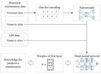
Deep learning is a group of machine learning algorithms [26]. It was originated from the artificial neural network [27] and has been researched in recent years. Deep learning does not rely on feature selection. The features which are barely relevant to the TBF will be allocated with a small weight. In other words, the weights of the input layer in a deep learning model can be used to represent the feature relevancy to the TBF. There are two targets in this study. Firstly, a deep learning model needs to be established to predict automobile TBF based on historical maintenance data and GIS data. Secondly, the impact of GIS features to the TBF need to be determined. In order to achieve this target, the following methodology is adopted.
Firstly, in order to process the nominal data (categorical variables) in historical maintenance data, one-hot encoding is necessary. However, when the number of categorical variables significantly surpasses the numeric variables, the dataset will become sparse and hard to be analysed [28]. Then, autoencoder, a deep learning algorithm, is used to train a neural network based on the one-hot encoded data in order to obtain low-dimension and robust data. The low-dimension and robust data is then concatenated with the rest numeric data in the dataset.
Secondly, with the coordinates (i.e. longitude and latitude) of an automobile workstation. The GIS data such as local geographical and climatic data can be collected. This data is then combined with the processed historical maintenance data as a new dataset. The new dataset is then normalised and randomised before it is used for modelling.
Thirdly, in the modelling stage, a deep learning model is established for automobile TBF prediction. The details about how to design a deep learning model were reported in our previous work [9]. In order to design a deep learning model, the types of a neural network need to be first determined according to the task and data type. In the next stage, the parameters of the deep learning model need to be selected and fine-tuned.
Finally, once the deep learning model is established, it is necessary to identify the impact of different features on TBF. Because the training process of deep learning cannot be monitored, it is hard to identify how features affect TBF. In a neural network, the weight of the input layer refers to the importance of the feature. Hence, extracting the weight of the
neural network’s input layer is helpful to identify the
relevancy between features and output. Fig.1 shows the flowchart of the methodology.
Fig. 1. The flowchart of the methodology. 4. Experimental Study
4.1.Experimental Setup and Data
In this study, a historical maintenance dataset of automobile engines is provided by a sizable fleet service company in the UK. Firstly, an understanding of the
company’s general information is necessary. There are a large
number of automobiles serving in the company, which include various types such as van and personal car. There are two maintenance management in the company, which are run-to-failure and scheduled check. Without the knowledge of predictive maintenance, it is hard to optimise the maintenance cost and spare part management. Hence, the company has a keen interest in when an automobile will break down and return to the workstation. If the TBF of an automobile can be predicted, the maintenance strategy can be modified to achieve better spare parts management and lower maintenance cost.
Secondly, the data collection method needs to be identified. The company has numerous workstations in different cities in the UK. When an automobile fails, it is returned to its belonging workstation. Then, the information of the failure such as failure time, type of automobile, and mileage is recorded. The historical maintenance dataset used in this study contains an excess of 10 thousand data entries in total. Each data entry represents the TBF and feature difference between the two maintenance record.
After the historical maintenance data was collected, the next step is to collect the GIS data. There are various types of GIS features might affect automobile TBF, which includes terrain, climate, traffic, etc. Among all these GIS data, climate data is relatively easy to access. In this study, climate data was collected according to the automobile workstation, before it was integrated with the historical maintenance data. In this study, the GIS data collected contains five climatic features. The climatic data used in this dataset is collected from the website of the Met Office, UK [29]. The collected climatic features can be categorised into two types: temperature relevant features and rainfall relevant features. As the weather in the UK is relatively mild from March to November and it
paper aims to establish a TBF prediction model for automobile using machine learning based on historical maintenance data and GIS data. Also, the impact of GIS data on automobile TBF is studied. The rest of the paper is organised as follows: The existing techniques in predictive maintenance and the cases of using GIS data for analysis are reviewed in Section 2. The methodology of how to establish a TBF prediction model using deep learning based on historical maintenance data and GIS data is reported in Section 3. Section 4 introduces an experimental study of TBF modelling using real-world data. Section 5 concludes the paper.
2. Literature Review
2.1.Statistical and Machine Learning Techniques in Predictive maintenance
The existing techniques in predictive maintenance can be categorised into two types, which are statistical methods and machine learning methods.
Parametric and semi-parametric methods are two types of well-known statistical methods in predictive maintenance. Parametric methods assume the lifetime of a machine follows a specific parametric distribution such as Weibull [12] and exponential [13]. The performance of parametric methods can be excellent when data generally follow a particular distribution. However, data distribution does not always fit the model perfectly and therefore the accuracy of parameter estimation cannot be always guaranteed. Accelerated failure time (AFT) model is an important parametric model which is used to analyse the accelerated or decelerated failure time. An AFT model was proposed to analyse the life-stress relationships for multiple types of stresses. The proposed model was developed based on n Log-Linear model. Its likelihood theory can be used to process censored data [14].
Nonparametric methods have been studied for decades. The most prevailing model is called the Cox proportional hazard model (Cox PHM) [15]. The Cox PHM and its variants are widely used in reliability analysis. It is well known for the flexibility in processing both censored and uncensored data. Many researchers have used the Cox PHM to study the reliability of a product at a certain time base on the variables relevant to the reliability [16]. The Standard Cox PHM can be used to analyse the relationship between reliability and time-independent covariates.
Besides statistical methods, machine learning techniques also have been investigated in predictive maintenance. Wei et al. [17] proposed a dynamic particle filter-support vector regression method to forecast system reliability. Nieto et al. [18] proposed a hybrid particle swarm optimisation support vector machine to predict the remaining useful life (RUL) of aircraft.
Because deep belief network does not rely on explicit model equations and domain knowledge, Zhao et al. [7] introduced a deep belief network to predict the RUL of bearing. A prognosis of defect propagation based recurrent neural network was designed to forecast the long-term prognostic machine reliability [8]. Both studies used data collected via sensors, while the former study focus on RUL
and the latter study focus on reliability. Zhang et al. [19] researched the prediction of RUL using deep learning. The raw sensor data is converted to health index using a single layer perceptron. Then the health index is used to train a bi-directional long-short-term memory network.
Wang et al. [20] proposed a conditional inference trees model to forecast the reliability of automobile engines. A tree-structured regression model was combined with Cox PHM in this study. The proposed tree model can offer straightforward interpretation reveal the significant attributes.
Both statistical and machine learning techniques are important in predictive maintenance. In the past, when the data size is small and low in dimension, statistical methods had been prevailing. In the era of big data, as the growing size and complexity of data, machine learning has gained increasing attention due to its excellent capability in data mining.
2.2.Machine Learning techniques in Processing GIS data
GIS is a powerful tool which has been widely used in spatial analysis. The knowledge obtained from GIS can be beneficial to decision making [11]. In the engineering field, Miles [21] proposed several examples of GIS modelling application in civil engineering. The benefits of using GIS in engineering modelling was summarized. Lee [22] proposed a logistic regression model to evaluate the hazard of landslides using GIS and remote sensing data. Several terrain features such as slope, curvature, and distance from drainage were selected to establish a logistic regression model.
In order to improve soil information for decision making, a predictive soil map was developed using digital soil mapping techniques. The soil profile data was collected, and a numeric classification was performed on the collected data to obtain soil taxa. Then, the soil taxa were spatially predicted and mapped using two machine learning algorithms, which are random forest and J48. Results indicated that random forest shows merits in modelling in comparison with J48 [23].
A spectral-spatial feature-based classification framework was proposed to extract spectral and spatial features. In this framework, a balanced local discriminant embedding algorithm is used to extract spectral features from hyperspectral datasets. A convolutional neural network was used to extract the spatial features. The spectral and spatial features are then stacked together to train a multiple-feature-based classifier [24].
Tehrani et al. [25] proposed a method that uses a weights-of evidence model and a support vector machine (SVM) technique to evaluate the correlation between flood occurrence and each conditioning factor. The performance of SVM based on four different kernels were identified. AUC (Area under the ROC Curve) was used to evaluate the algorithm performance. Results can be helpful to local government about optimising flood mitigation strategies.
2.3.A Brief Summary
From literature, it is obvious that various techniques in statistics and machine learning have been investigated in
predictive maintenance. Recently, in order to obtain knowledge for decision making, researchers have studied GIS data using machine learning techniques. However, to the best of our knowledge, there are no studies in predictive maintenance using GIS data. As we all know, automobile TBF is affected by different GIS factors such as climate, terrain and traffic condition. If GIS data can be introduced into TBF modelling and identified how its impact on automobile TBF, fleet management companies can adjust their maintenance strategy to lower the maintenance cost.
3. Methodology
Deep learning is a group of machine learning algorithms [26]. It was originated from the artificial neural network [27] and has been researched in recent years. Deep learning does not rely on feature selection. The features which are barely relevant to the TBF will be allocated with a small weight. In other words, the weights of the input layer in a deep learning model can be used to represent the feature relevancy to the TBF. There are two targets in this study. Firstly, a deep learning model needs to be established to predict automobile TBF based on historical maintenance data and GIS data. Secondly, the impact of GIS features to the TBF need to be determined. In order to achieve this target, the following methodology is adopted.
Firstly, in order to process the nominal data (categorical variables) in historical maintenance data, one-hot encoding is necessary. However, when the number of categorical variables significantly surpasses the numeric variables, the dataset will become sparse and hard to be analysed [28]. Then, autoencoder, a deep learning algorithm, is used to train a neural network based on the one-hot encoded data in order to obtain low-dimension and robust data. The low-dimension and robust data is then concatenated with the rest numeric data in the dataset.
Secondly, with the coordinates (i.e. longitude and latitude) of an automobile workstation. The GIS data such as local geographical and climatic data can be collected. This data is then combined with the processed historical maintenance data as a new dataset. The new dataset is then normalised and randomised before it is used for modelling.
Thirdly, in the modelling stage, a deep learning model is established for automobile TBF prediction. The details about how to design a deep learning model were reported in our previous work [9]. In order to design a deep learning model, the types of a neural network need to be first determined according to the task and data type. In the next stage, the parameters of the deep learning model need to be selected and fine-tuned.
Finally, once the deep learning model is established, it is necessary to identify the impact of different features on TBF. Because the training process of deep learning cannot be monitored, it is hard to identify how features affect TBF. In a neural network, the weight of the input layer refers to the importance of the feature. Hence, extracting the weight of the
neural network’s input layer is helpful to identify the
relevancy between features and output. Fig.1 shows the flowchart of the methodology.
Fig. 1. The flowchart of the methodology. 4. Experimental Study
4.1.Experimental Setup and Data
In this study, a historical maintenance dataset of automobile engines is provided by a sizable fleet service company in the UK. Firstly, an understanding of the
company’s general information is necessary. There are a large
number of automobiles serving in the company, which include various types such as van and personal car. There are two maintenance management in the company, which are run-to-failure and scheduled check. Without the knowledge of predictive maintenance, it is hard to optimise the maintenance cost and spare part management. Hence, the company has a keen interest in when an automobile will break down and return to the workstation. If the TBF of an automobile can be predicted, the maintenance strategy can be modified to achieve better spare parts management and lower maintenance cost.
Secondly, the data collection method needs to be identified. The company has numerous workstations in different cities in the UK. When an automobile fails, it is returned to its belonging workstation. Then, the information of the failure such as failure time, type of automobile, and mileage is recorded. The historical maintenance dataset used in this study contains an excess of 10 thousand data entries in total. Each data entry represents the TBF and feature difference between the two maintenance record.
After the historical maintenance data was collected, the next step is to collect the GIS data. There are various types of GIS features might affect automobile TBF, which includes terrain, climate, traffic, etc. Among all these GIS data, climate data is relatively easy to access. In this study, climate data was collected according to the automobile workstation, before it was integrated with the historical maintenance data. In this study, the GIS data collected contains five climatic features. The climatic data used in this dataset is collected from the website of the Met Office, UK [29]. The collected climatic features can be categorised into two types: temperature relevant features and rainfall relevant features. As the weather in the UK is relatively mild from March to November and it
becomes rainy and cold from December to February. The high humidity and low temperature might have a negative impact on the health of an automobile. Hence, the average climatic data from December to February was adopted in this study.
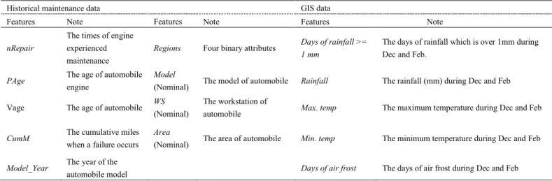
The feature description is shown in Table 1. The historical maintenance dataset contains seven features which are deemed highly relevant to TBF. Among these features, four of them are numeric, while the rest three of them are the nominal type of data. For the GIS data, all the climatic features are numeric.
Feature selection is an important process for machine
learning algorithms. In this case, two prevailing feature selection algorithms which are CfsSubEval [30] and
WrapperSubEval [31] are used. Results indicated that only
three features out of 31 features in total are recommended by the algorithms. It is hard to identify the relevancy between the rest 28 features and TBF. Because deep learning has excellent capability in identifying features relevancy. All 31 features were used for modelling. The impact of features was studied after the modelling stage via extracting the weights of the first layer in deep learning model.
Table 1. The features description.
Historical maintenance data GIS data
Features Note Features Note Features Note
nRepair
The times of engine experienced maintenance
Regions Four binary attributes Days of rainfall >= 1 mm The days of rainfall which is over 1mm during Dec and Feb.
PAge The age of automobile engine
Model
(Nominal) The model of automobile Rainfall The rainfall (mm) during Dec and Feb Vage The age of automobile WS
(Nominal)
The workstation of
automobile Max. temp The maximum temperature during Dec and Feb CumM The cumulative miles
when a failure occurs Area
(Nominal) The area of automobile Min. temp The minimum temperature during Dec and Feb Model_Year The year of the
automobile model Days of air frost The days of air frost during Dec and Feb Secondly, the nominal data was transformed using one-hot
encoding [32]. The data generated via one-hot encoding increased the dimension of the nominal data from 4 to 164, which dramatically increase the data sparsity. In order to lower the data sparsity, autoencoder [33], a deep learning algorithm, was employed in this study to encode the sparse data to robust representation. The autoencoder model consists of three fully-connected layers, which the number of node in input and output layer was set at 164 (the dimension of one-hot encoding attributes) and the number of node in hidden layer was set at 16 (the required dimension of the encoded data). With the help of autoencoder, the dimension of autoencoder decreased from 164 to 16. The data generated by autoencoder was then concatenated with the rest numeric data to be a new dataset. The new dataset contains 31 features and in excess of 10 thousand data entries in total. Figure 2 shows the structure of the autoencoder.
Autoencoder is trained using back-propagation algorithm. The input vector of autoencoder is denoted as 𝑥𝑥. The features learned by the encoder, also known as code, is denoted as 𝑧𝑧. The relation between 𝑥𝑥 and 𝑧𝑧can be denoted as:
𝑧𝑧 = 𝜎𝜎(𝑊𝑊𝑥𝑥 + 𝑏𝑏) (1) where W is the weight matrix between the input layer and the hidden layer, b is the bias, and the σ() is the activation function.
The features 𝑧𝑧 learned from the hidden layer is then used to construct a vector 𝑥𝑥′ which is expected the same as vector 𝑥𝑥. The relationship between 𝑥𝑥′ and 𝑧𝑧 can be represented as:
𝑥𝑥′= 𝜎𝜎(𝑊𝑊′𝑧𝑧 + 𝑏𝑏′) (2)
where 𝑊𝑊′is the weight matrix between the input layer and the hidden layer, 𝑏𝑏′ is the bias, and the 𝜎𝜎()is the activation function.
Thirdly, the new dataset was normalised to increase data integrity [34]. Specifically, all the data was scaled into the range from 0 to 1. Finally, the dataset was randomised. The shuffle of the dataset can avoid some local patterns to be learned by an algorithm, which may damage the algorithm performance.
In the evaluation stage, 10-fold cross-validation was adopted to obtain a comprehensive result. In order to reveal the algorithm performance, Root Mean Square Error (RMSE) was adopted as an evaluation metric. RMSE is a metric that measures the difference between the predicted and actual values.
Fig. 2. The structure of autoencoder.
4.2.Model Setup
In our previous study, the experimental results indicated deep learning shows merits in automobile TBF modelling in comparison with several prevailing machine learning algorithms [9]. In this study, we mainly focused on the impact of GIS data on TBF modelling. A deep learning algorithm which is a deep neural network (DNN) and three prevailing machine learning algorithms, which are Bayesian regression (BR), random forest [35] k-nearest neighbours (k-NN), was used to establish TBF prediction model based on the clean dataset, separately. The models were established using the Python language.
In order to build a neural network, there are several elements need to be determined: layer, activation function, loss function and optimizer. Firstly, the DNN designed in this study consists of fully connected layers and drop-out layers. The fully connected layer is the basic layer of deep learning. Drop-out layer is used to avoid overfitting by randomly cutting a certain ratio of connection in the training process [36]. Secondly, the activation function is used to process the input of a neuron. Rectified Linear Units (ReLU) is a popular activation function in deep learning owning to its biological motivation and mathematical justifications [37]. Thirdly, the optimizer is used to optimise the training process of deep learning. Adam is a prevailing optimizer in deep learning [38] and it was adopted as the optimizer of the DNN. Finally, the mean square error was adopted as the loss function due to its popularity in the regression task.
The parameters setting of DNN is also essential to algorithm performance. After several trials, the number of layers in DNN was set at four (exclude two drop-out layers) and the node of each hidden layer in DNN was set at 1000. The ratio of drop-out was set at 20%. The batch size and training epochs of DNN were set at 50 and 45, respectively. The learning rate was set at 0.001. Fig. 3 shows the structure of DNN.
Fig. 3. The structure of DNN.
4.3.Deep Learning Modelling Based on Historical
Maintenance Data and GIS Data
In this study, in order to reveal the impact of GIS data on TBF modelling, two groups of machine learning models were trained based on different datasets. The models in the first
group were only trained based on the historical maintenance data, while the models in the second group were trained based on the combination of historical maintenance data and GIS data. The parameters setting of DNN is the same for both groups. The results of modelling were obtained using 10-fold cross-validation. Table 2 shows the results of modelling. Table 2. The results of TBF modelling using DNN.
RMSE of Historical maintenance data (days)
RMSE of Historical maintenance data+ GIS data (days)
DNN 366.73 363.07
BR 401.73 402.65
RF 380.09 376.65
k-NN 398.91 397.64
It can be seen from the results that DNN and RF show better performance with the help of GIS data, while the RMSE of BR and k-NN are barely changed. Among the four algorithms, DNN achieved the lowest RMSE which is 363.07 days.
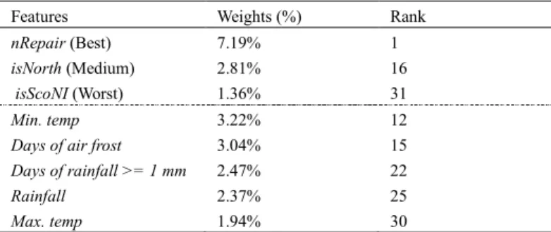
In order to identify the relevancy between GIS features and automobile TBF, the weights of the input layer in DNN was extracted, normalised, and ranked. Table 3 shows the details of the weights and rank of GIS features in all the features.
It can be seen from the results that the weights and rank of the GIS features rank at different levels. The most relevant feature in the dataset takes 7.19% of the weights in the input layer of DNN, while the most irrelevant feature in the dataset takes mere 1.94% of the weights. The most relevant GIS feature is the Min. temp, which weight is 3.22%. The second and third relevant GIS features are Days of air frost and Days
of rainfall >= 1 mm, which takes 3.04% and 2.47%,
respectively. Rainfall and Max. temp occupy the least weight among all the features.
Table 3. The weights and rank of the GIS features.
Features Weights (%) Rank
nRepair (Best) 7.19% 1
isNorth (Medium) 2.81% 16
isScoNI (Worst) 1.36% 31
Min. temp 3.22% 12
Days of air frost 3.04% 15
Days of rainfall >= 1mm 2.47% 22
Rainfall 2.37% 25
Max. temp 1.94% 30 4.4.Discussion
In this study, four algorithms were used for TBF modelling. Feature selection is an important process before modelling using machine learning algorithms. Because the results of the prevailing feature selection algorithms do not offer explicit knowledge, the algorithm performance of BR, RF and k-NN might be compromised. The deep neural network is an algorithm which is able to identify the relevancy between inputs and output during the training process. It is reasonable that it achieved the lowest RMSE. In order to identify the impact of GIS features on automobile TBF, the weights of DNN was used to identify the impact of GIS data. Results
becomes rainy and cold from December to February. The high humidity and low temperature might have a negative impact on the health of an automobile. Hence, the average climatic data from December to February was adopted in this study.
The feature description is shown in Table 1. The historical maintenance dataset contains seven features which are deemed highly relevant to TBF. Among these features, four of them are numeric, while the rest three of them are the nominal type of data. For the GIS data, all the climatic features are numeric.
Feature selection is an important process for machine
learning algorithms. In this case, two prevailing feature selection algorithms which are CfsSubEval [30] and
WrapperSubEval [31] are used. Results indicated that only
three features out of 31 features in total are recommended by the algorithms. It is hard to identify the relevancy between the rest 28 features and TBF. Because deep learning has excellent capability in identifying features relevancy. All 31 features were used for modelling. The impact of features was studied after the modelling stage via extracting the weights of the first layer in deep learning model.
Table 1. The features description.
Historical maintenance data GIS data
Features Note Features Note Features Note
nRepair
The times of engine experienced maintenance
Regions Four binary attributes Days of rainfall >= 1 mm The days of rainfall which is over 1mm during Dec and Feb.
PAge The age of automobile engine
Model
(Nominal) The model of automobile Rainfall The rainfall (mm) during Dec and Feb Vage The age of automobile WS
(Nominal)
The workstation of
automobile Max. temp The maximum temperature during Dec and Feb CumM The cumulative miles
when a failure occurs Area
(Nominal) The area of automobile Min. temp The minimum temperature during Dec and Feb Model_Year The year of the
automobile model Days of air frost The days of air frost during Dec and Feb Secondly, the nominal data was transformed using one-hot
encoding [32]. The data generated via one-hot encoding increased the dimension of the nominal data from 4 to 164, which dramatically increase the data sparsity. In order to lower the data sparsity, autoencoder [33], a deep learning algorithm, was employed in this study to encode the sparse data to robust representation. The autoencoder model consists of three fully-connected layers, which the number of node in input and output layer was set at 164 (the dimension of one-hot encoding attributes) and the number of node in hidden layer was set at 16 (the required dimension of the encoded data). With the help of autoencoder, the dimension of autoencoder decreased from 164 to 16. The data generated by autoencoder was then concatenated with the rest numeric data to be a new dataset. The new dataset contains 31 features and in excess of 10 thousand data entries in total. Figure 2 shows the structure of the autoencoder.
Autoencoder is trained using back-propagation algorithm. The input vector of autoencoder is denoted as 𝑥𝑥. The features learned by the encoder, also known as code, is denoted as 𝑧𝑧. The relation between 𝑥𝑥 and 𝑧𝑧can be denoted as:
𝑧𝑧 = 𝜎𝜎(𝑊𝑊𝑥𝑥 + 𝑏𝑏) (1) where W is the weight matrix between the input layer and the hidden layer, b is the bias, and the σ() is the activation function.
The features 𝑧𝑧 learned from the hidden layer is then used to construct a vector 𝑥𝑥′ which is expected the same as vector 𝑥𝑥. The relationship between 𝑥𝑥′ and 𝑧𝑧 can be represented as:
𝑥𝑥′= 𝜎𝜎(𝑊𝑊′𝑧𝑧 + 𝑏𝑏′) (2)
where 𝑊𝑊′is the weight matrix between the input layer and the hidden layer, 𝑏𝑏′ is the bias, and the 𝜎𝜎()is the activation function.
Thirdly, the new dataset was normalised to increase data integrity [34]. Specifically, all the data was scaled into the range from 0 to 1. Finally, the dataset was randomised. The shuffle of the dataset can avoid some local patterns to be learned by an algorithm, which may damage the algorithm performance.
In the evaluation stage, 10-fold cross-validation was adopted to obtain a comprehensive result. In order to reveal the algorithm performance, Root Mean Square Error (RMSE) was adopted as an evaluation metric. RMSE is a metric that measures the difference between the predicted and actual values.
Fig. 2. The structure of autoencoder.
4.2.Model Setup
In our previous study, the experimental results indicated deep learning shows merits in automobile TBF modelling in comparison with several prevailing machine learning algorithms [9]. In this study, we mainly focused on the impact of GIS data on TBF modelling. A deep learning algorithm which is a deep neural network (DNN) and three prevailing machine learning algorithms, which are Bayesian regression (BR), random forest [35] k-nearest neighbours (k-NN), was used to establish TBF prediction model based on the clean dataset, separately. The models were established using the Python language.
In order to build a neural network, there are several elements need to be determined: layer, activation function, loss function and optimizer. Firstly, the DNN designed in this study consists of fully connected layers and drop-out layers. The fully connected layer is the basic layer of deep learning. Drop-out layer is used to avoid overfitting by randomly cutting a certain ratio of connection in the training process [36]. Secondly, the activation function is used to process the input of a neuron. Rectified Linear Units (ReLU) is a popular activation function in deep learning owning to its biological motivation and mathematical justifications [37]. Thirdly, the optimizer is used to optimise the training process of deep learning. Adam is a prevailing optimizer in deep learning [38] and it was adopted as the optimizer of the DNN. Finally, the mean square error was adopted as the loss function due to its popularity in the regression task.
The parameters setting of DNN is also essential to algorithm performance. After several trials, the number of layers in DNN was set at four (exclude two drop-out layers) and the node of each hidden layer in DNN was set at 1000. The ratio of drop-out was set at 20%. The batch size and training epochs of DNN were set at 50 and 45, respectively. The learning rate was set at 0.001. Fig. 3 shows the structure of DNN.
Fig. 3. The structure of DNN.
4.3.Deep Learning Modelling Based on Historical
Maintenance Data and GIS Data
In this study, in order to reveal the impact of GIS data on TBF modelling, two groups of machine learning models were trained based on different datasets. The models in the first
group were only trained based on the historical maintenance data, while the models in the second group were trained based on the combination of historical maintenance data and GIS data. The parameters setting of DNN is the same for both groups. The results of modelling were obtained using 10-fold cross-validation. Table 2 shows the results of modelling. Table 2. The results of TBF modelling using DNN.
RMSE of Historical maintenance data (days)
RMSE of Historical maintenance data+ GIS data (days)
DNN 366.73 363.07
BR 401.73 402.65
RF 380.09 376.65
k-NN 398.91 397.64
It can be seen from the results that DNN and RF show better performance with the help of GIS data, while the RMSE of BR and k-NN are barely changed. Among the four algorithms, DNN achieved the lowest RMSE which is 363.07 days.
In order to identify the relevancy between GIS features and automobile TBF, the weights of the input layer in DNN was extracted, normalised, and ranked. Table 3 shows the details of the weights and rank of GIS features in all the features.
It can be seen from the results that the weights and rank of the GIS features rank at different levels. The most relevant feature in the dataset takes 7.19% of the weights in the input layer of DNN, while the most irrelevant feature in the dataset takes mere 1.94% of the weights. The most relevant GIS feature is the Min. temp, which weight is 3.22%. The second and third relevant GIS features are Days of air frost and Days
of rainfall >= 1 mm, which takes 3.04% and 2.47%,
respectively. Rainfall and Max. temp occupy the least weight among all the features.
Table 3. The weights and rank of the GIS features.
Features Weights (%) Rank
nRepair (Best) 7.19% 1
isNorth (Medium) 2.81% 16
isScoNI (Worst) 1.36% 31
Min. temp 3.22% 12
Days of air frost 3.04% 15
Days of rainfall >= 1mm 2.47% 22
Rainfall 2.37% 25
Max. temp 1.94% 30 4.4.Discussion
In this study, four algorithms were used for TBF modelling. Feature selection is an important process before modelling using machine learning algorithms. Because the results of the prevailing feature selection algorithms do not offer explicit knowledge, the algorithm performance of BR, RF and k-NN might be compromised. The deep neural network is an algorithm which is able to identify the relevancy between inputs and output during the training process. It is reasonable that it achieved the lowest RMSE. In order to identify the impact of GIS features on automobile TBF, the weights of DNN was used to identify the impact of GIS data. Results
indicate that the introduction of GIS data is beneficial to TBF modelling using DNN. It is evident that automobile TBF is sensitive to the cold weather relevant features such as Min. temp and Days of air frost. In contrast, automobile TBF is not very sensitive to the humidity relevant features such as Days of rainfall >= 1 mm and Rainfall. With this knowledge, fleet management companies can adjust their maintenance strategy. For example, for the workshop in the cold area, the automobiles need to check more frequently. The GIS data used in this study is only climatic data. In the future, more data relevant to automobile TBF such as terrain data and traffic data will be collected and studied their impact on TBF. 5. Conclusions
Predictive maintenance is an essential topic for fleet management. In this study, the method of how to introduce GIS data into TBF modelling and identify their impact on TBF has been introduced. An experimental study is introduced to machine learning algorithms to establish TBF prediction models based on historical maintenance data and GIS data. Experimental results indicate that better TBF prediction can be achieved with the help of GIS data. Besides, the impact of GIS data on TBF is identified. The knowledge derived from this study can be beneficial to fleet management companies to optimise their maintenance strategy.
References
[1] Takata S, Kirnura F, van Houten FJ, Westkamper E, Shpitalni M, Ceglarek D, Lee J, Maintenance: Changing role in life cycle management, CIRP Annals-Manufacturing Technology, 53; 2004. 643-655.
[2] Shyjith K, Ilangkumaran M, Kumanan S, Multi-criteria decision-making approach to evaluate optimum maintenance strategy in textile industry, Journal of Quality in Maintenance Engineering, 14; 2008. 375-386. [3] Zhang Y, Liu Q, Reliability-based design of automobile components,
Proceedings of the Institution of Mechanical Engineers, Part D: Journal of Automobile Engineering, 216; 2002. 455-471.
[4] Mobley RK, An introduction to predictive maintenance, Elsevier, 2002. [5] Cresci J-P, Lortie P, Bhattacharya K, Machine learning: A turning point
for predictive maintenance?, in, URL:
https://www.oliverwyman.com/content/dam/oliver-wyman/v2/publications/2017/sep/Predictive_Maintenance.pdf. 2017, pp. 1-5.
[6] LeCun Y, Bengio Y, Hinton G, Deep learning, Nature, 521; 2015. 436-444.
[7] Zhao G, Liu X, Zhang B, Zhang G, Niu G, Hu C, Bearing health condition prediction using deep belief network, Annual Conference of the Prognostics and Health Management Society; 2017.
[8] Malhi A, Yan R, Gao RX, Prognosis of defect propagation based on recurrent neural networks, IEEE Transactions on Instrumentation and Measurement, 60; 2011. 703-711.
[9] Chen C, Liu Y, Sun X, Wang S, Di Cairano-Gilfedder C, Titmus S, Syntetos AA, Reliability analysis using deep learning, in: ASME 2018 International Design Engineering Technical Conferences and Computers and Information in Engineering Conference, American Society of Mechanical Engineers. 2018, pp. V01BT02A040-V001BT002A040. [10] Carnero M, An evaluation system of the setting up of predictive
maintenance programmes, Reliability Engineering & System Safety, 91; 2006. 945-963.
[11] Rikalovic A, Cosic I, Lazarevic D, Gis based multi-criteria analysis for industrial site selection, Procedia Engineering, 69; 2014. 1054-1063. [12] Xie M, Lai CD, Reliability analysis using an additive weibull model with
bathtub-shaped failure rate function, Reliability Engineering & System Safety, 52; 1996. 87-93.
[13] Grubbs FE, Approximate fiducial bounds on reliability for the two parameter negative exponential distribution, Technometrics, 13; 1971. 873-876.
[14] Mettas A, Modeling and analysis for multiple stress-type accelerated life data, in: Reliability and Maintainability Symposium, 2000. Proceedings. Annual, IEEE, 2000, pp. 138-143.
[15] Cox DR, Regression models and life-tables, in: Breakthroughs in statistics, Springer, 1992, pp. 527-541.
[16] Kumar D, Klefsjö B, Proportional hazards model: A review, Reliability Engineering & System Safety, 44; 1994. 177-188.
[17] Wei Z, Tao T, ZhuoShu D, Zio E, A dynamic particle filter-support vector regression method for reliability prediction, Reliability Engineering & System Safety, 119; 2013. 109-116.
[18] Nieto PG, García-Gonzalo E, Lasheras FS, de Cos Juez FJ, Hybrid pso– svm-based method for forecasting of the remaining useful life for aircraft engines and evaluation of its reliability, Reliability Engineering & System Safety, 138; 2015. 219-231.
[19] Zhang J, Wang P, Yan R, Gao RX, Deep learning for improved system remaining life prediction, Procedia CIRP, 72; 2018. 1033-1038.
[20] Wang S, Liu Y, Cairano-Gilfedder CD, Titmus S, Naim MM, Syntetos AA, Reliability analysis for automobile engines: Conditional inference trees, Procedia CIRP, 72; 2018. 1392-1397.
[21] Miles SB, Ho CL, Applications and issues of gis as tool for civil engineering modeling, Journal of computing in civil engineering, 13; 1999. 144-152.
[22] Lee S, Application of logistic regression model and its validation for landslide susceptibility mapping using gis and remote sensing data, International Journal of Remote Sensing, 26; 2005. 1477-1491.
[23] Massawe BH, Subburayalu SK, Kaaya AK, Winowiecki L, Slater BK, Mapping numerically classified soil taxa in kilombero valley, tanzania using machine learning, Geoderma, 311; 2018. 143-148.
[24] Zhao W, Du S, Spectral–spatial feature extraction for hyperspectral image classification: A dimension reduction and deep learning approach, IEEE Transactions on Geoscience and Remote Sensing, 54; 2016. 4544-4554.
[25] Tehrany MS, Pradhan B, Jebur MN, Flood susceptibility mapping using a novel ensemble weights-of-evidence and support vector machine models in gis, Journal of hydrology, 512; 2014. 332-343.
[26] Deng L, Yu D, Deep learning: Methods and applications, Foundations and Trends® in Signal Processing, 7; 2014. 197-387.
[27] Bengio Y, Learning deep architectures for ai, Foundations and trends® in Machine Learning, 2; 2009. 1-127.
[28] Hosseini-Asl E, Zurada JM, Nasraoui O, Deep learning of part-based representation of data using sparse autoencoders with nonnegativity constraints, IEEE transactions on neural networks and learning systems, 27; 2016. 2486-2498.
[29] Weather and climate change-met office, in, 2018.
[30] Shilbayeh S, Vadera S, Feature selection in meta learning framework, in: Science and Information Conference; SAI., 2014, IEEE, 2014, pp. 269-275.
[31] Guyon I, Elisseeff A, An introduction to variable and feature selection, Journal of machine learning research, 3; 2003. 1157-1182.
[32] Breiman L, Classification and regression trees, Routledge, 2017. [33] Han K, Li C, Shi X, Autoencoder feature selector, arXiv preprint
arXiv:1710.08310, 2017.
[34] Codd EF, A relational model of data for large shared data banks, Communications of the ACM, 13; 1970. 377-387.
[35] Ullah I, Yang F, Khan R, Liu L, Yang H, Gao B, Sun K, Predictive maintenance of power substation equipment by infrared thermography using a machine-learning approach, Energies, 10; 2017. 1987.
[36] Srivastava N, Hinton G, Krizhevsky A, Sutskever I, Salakhutdinov R, Dropout: A simple way to prevent neural networks from overfitting, The Journal of Machine Learning Research, 15; 2014. 1929-1958.
[37] Hahnloser RH, Sarpeshkar R, Mahowald MA, Douglas RJ, Seung HS, Digital selection and analogue amplification coexist in a cortex-inspired silicon circuit, Nature, 405; 2000. 947.
[38] Kingma DP, Ba J, Adam: A method for stochastic optimization, arXiv preprint arXiv:1412.6980, 2014.